Category Archives: Multiple Cloud Layers

Fog over the southeast US

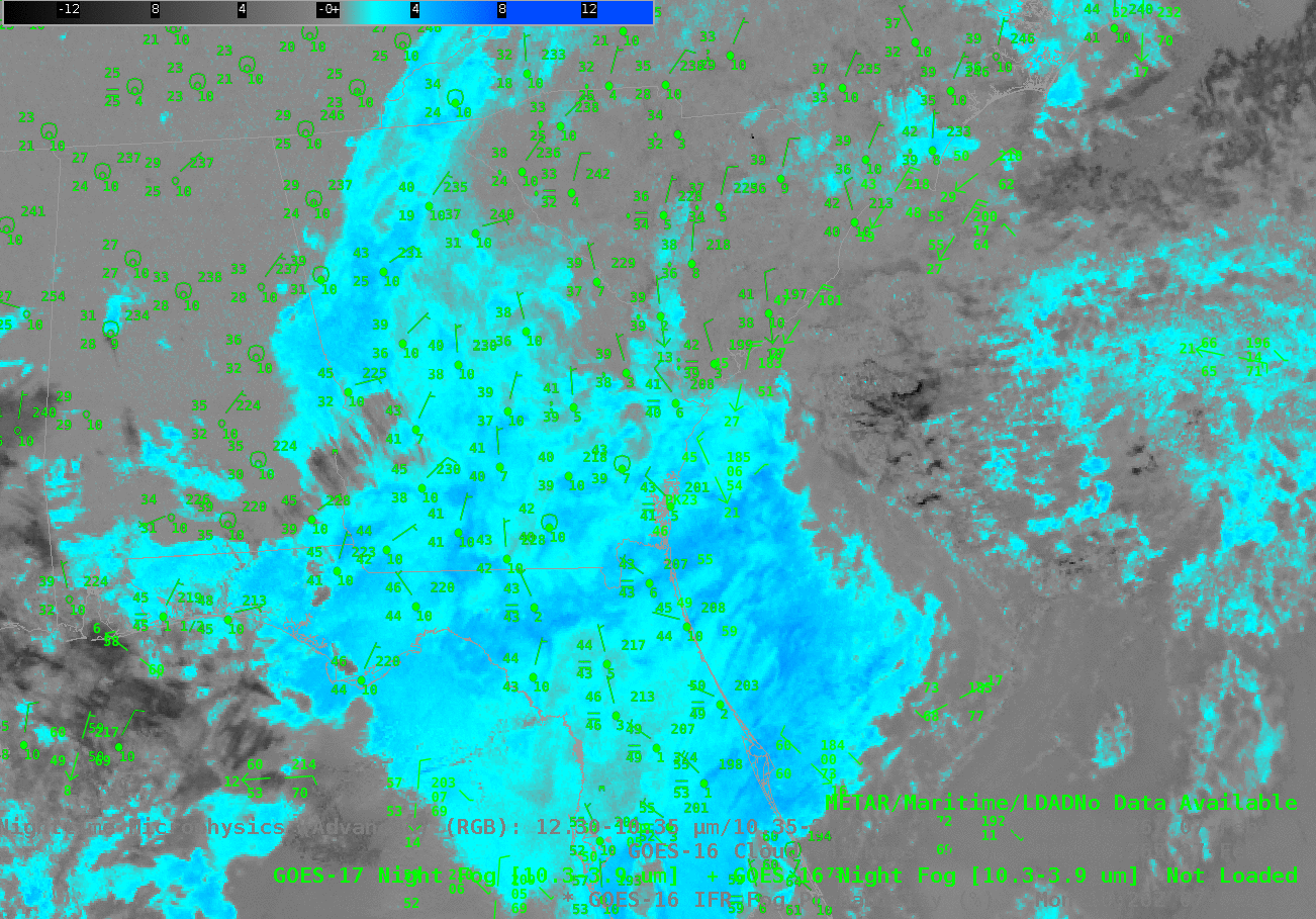
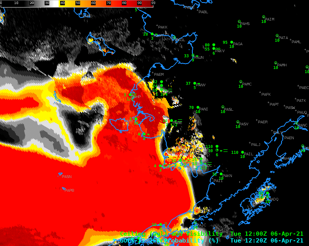
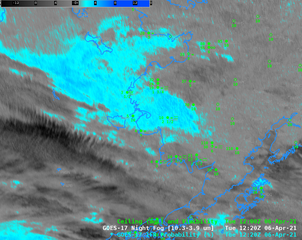
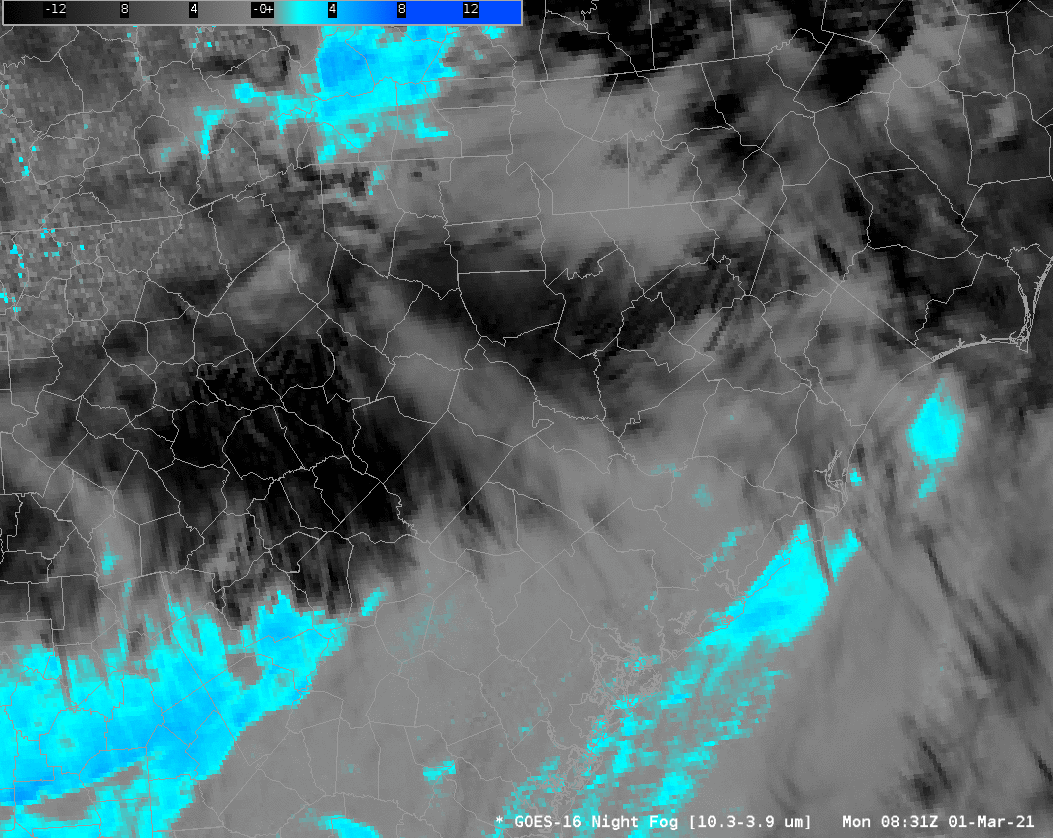
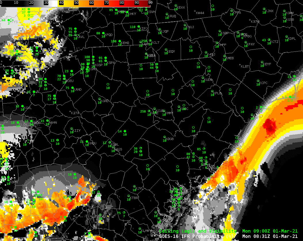
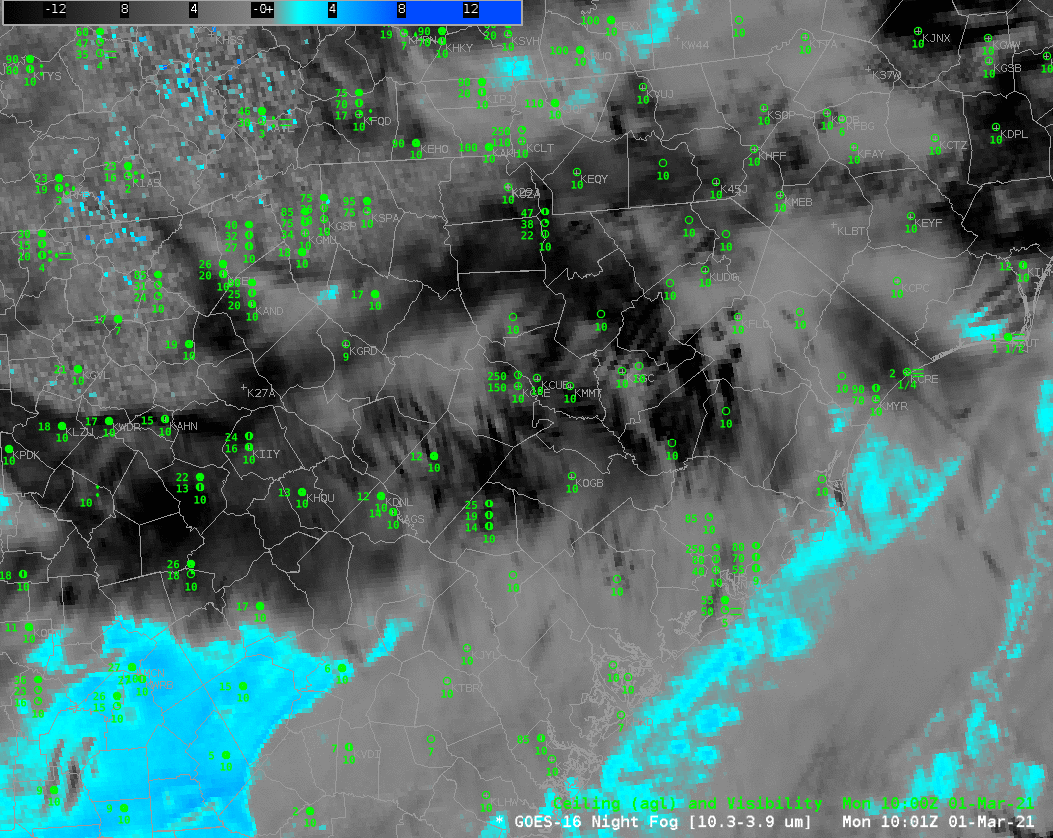
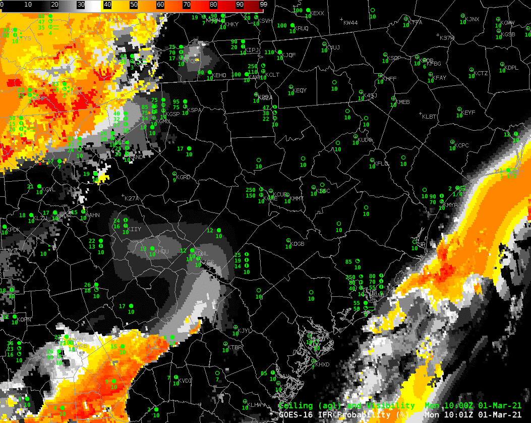
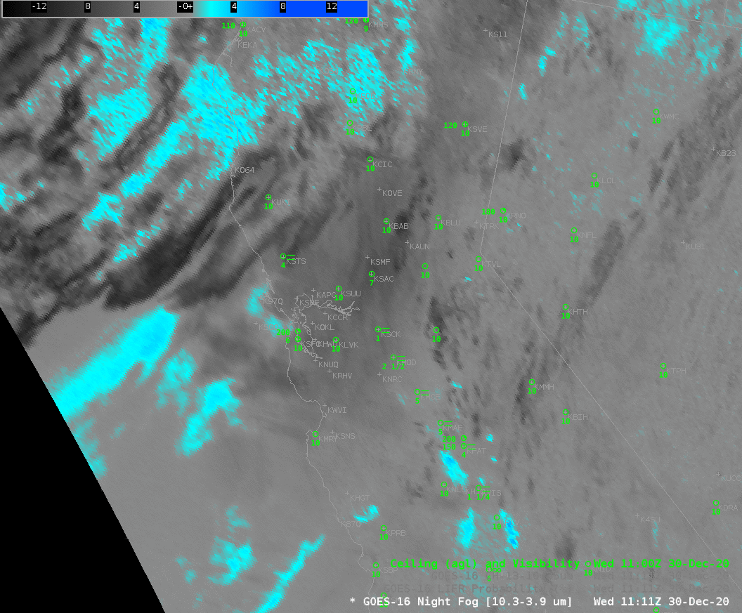
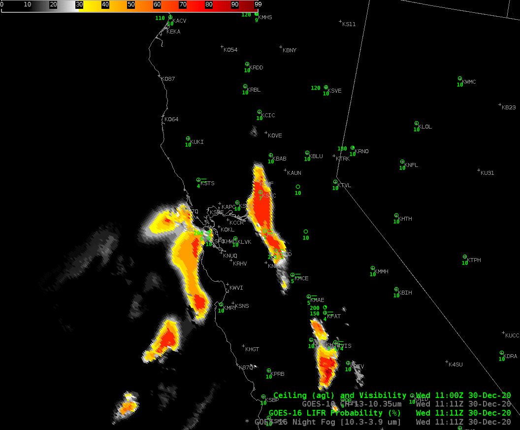
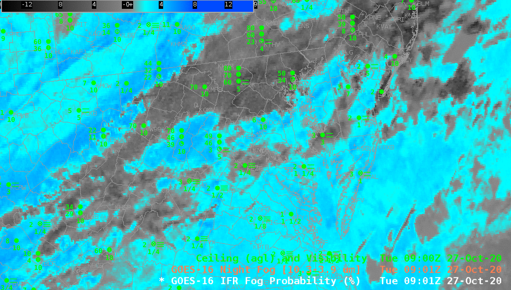
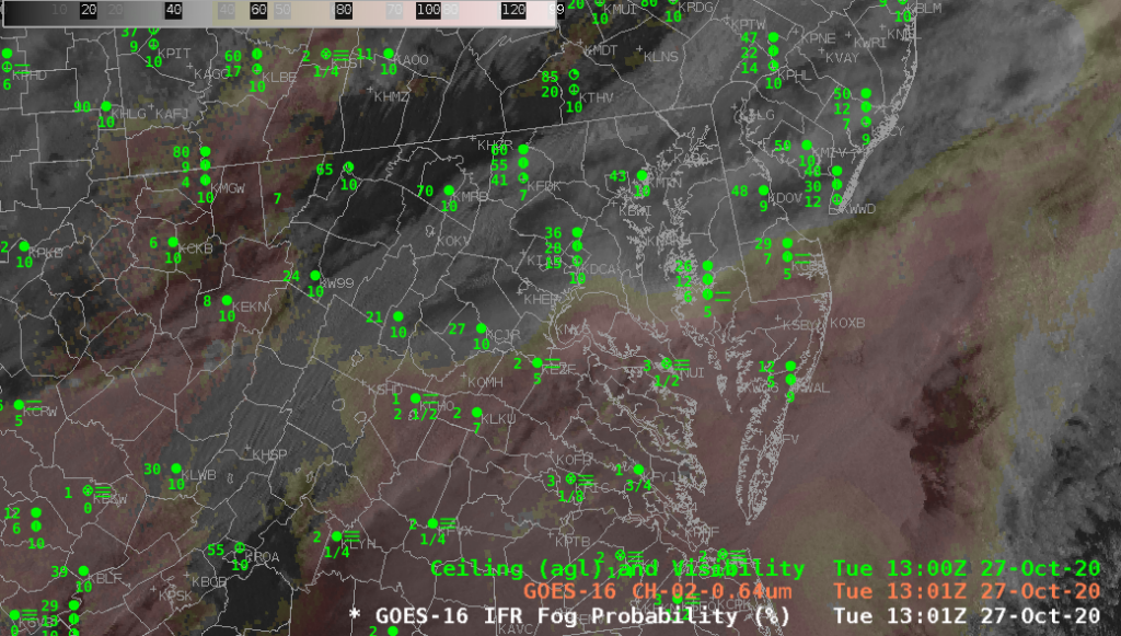
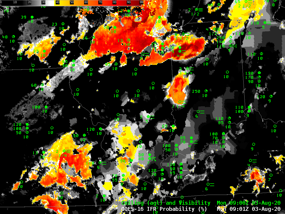
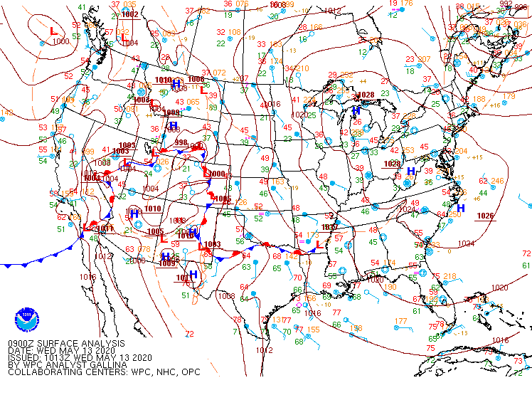
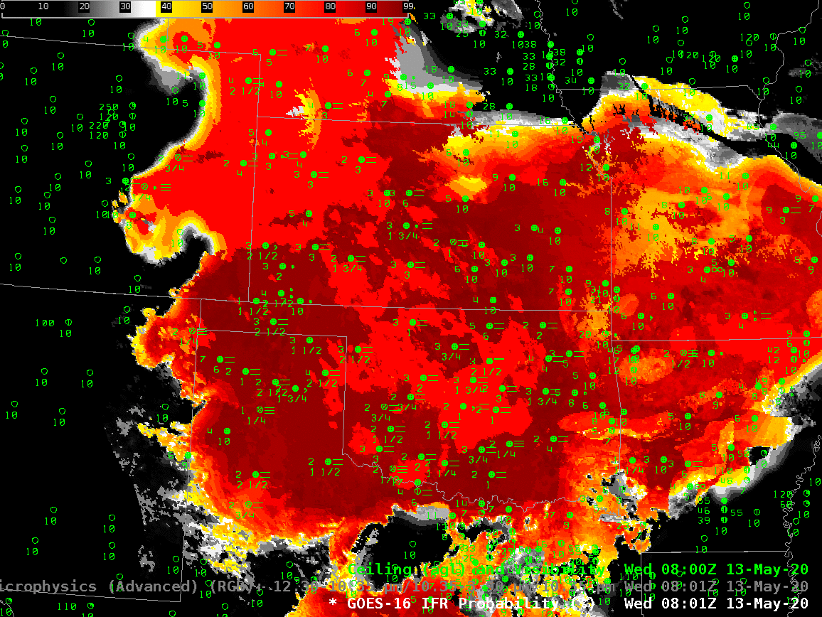
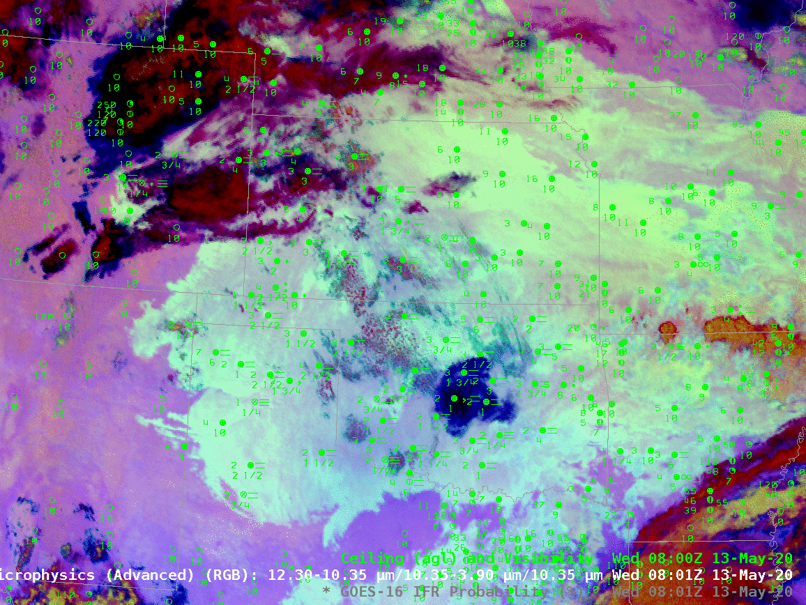
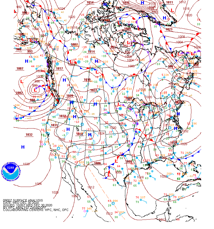
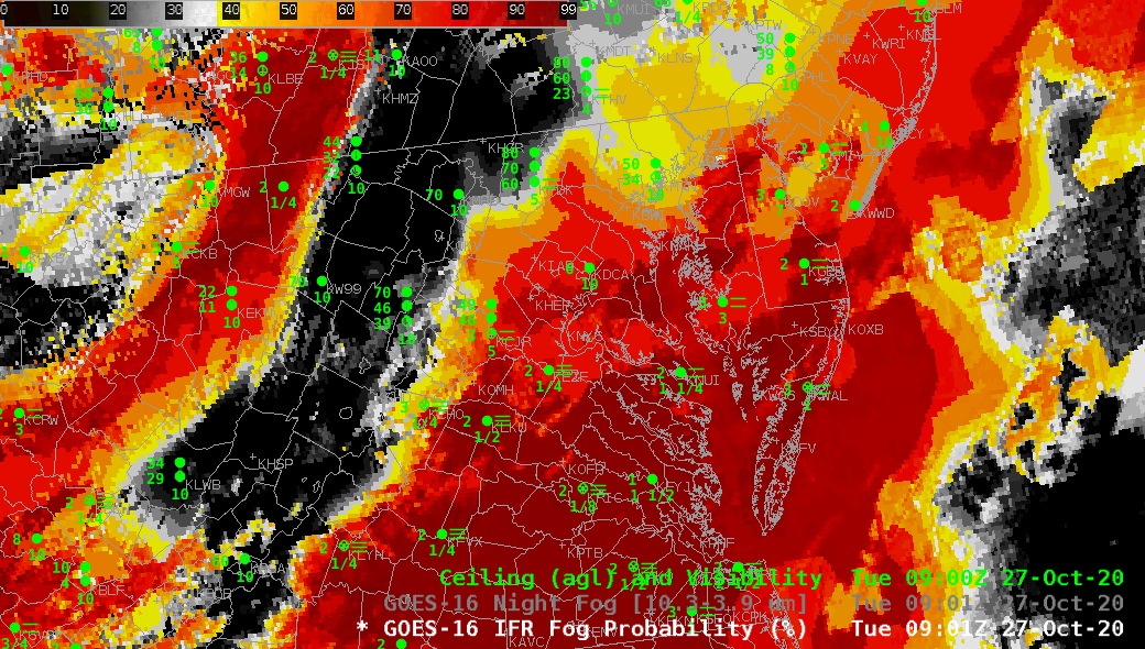
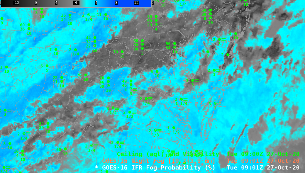
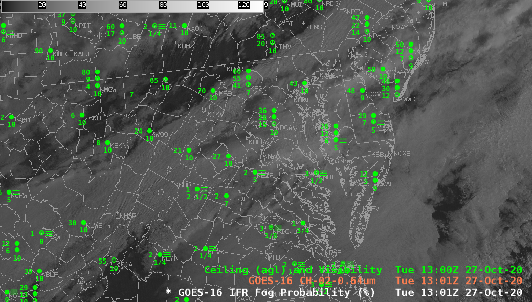
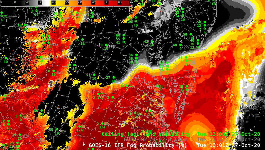
Low pressure just off the coast of South Carolina (0900 UTC map analysis) brought wide-spread fog and low ceilings to the southeastern United States on 7 February. The toggle below shows the Night Fog Brightness Temperature Difference (BTD, 10.3 µm – 3.9 µm) field that is often used to highlight regions where clouds made up of water droplets are widespread. The night time microphysics RGB includes as its green component the Night Fog BTD, and the correlation between the blue/cyan enhancement in the BTD and the cyan/yellowish color in the RGB is obvious. A challenge in using those two fields for low fog/stratus detection arises where multiple cloud layers might exist such that the BTD is not highlighting low cloud — because mid-level or high clouds block the satellite view of low clouds. This shortcoming is mitigated in IFR Probability fields by including information (from the Rapid Refresh model) on low-level saturation. Thus, IFR Probability fields suggest a greater likelihood for low clouds over coastal South Carolina (for example). If low-level saturation is *not* indicated in the model, IFR Probabilities will show minimal values, as over central Georgia (near Atlanta, especially), for example.

GOES-16 Night Fog Brightness Temperature Difference (10.3 µm – 3.9 µm), Night time microphysics RGB, and GOES-R IFR Probability, 1026 UTC on 7 February 2022 (Click to enlarge)

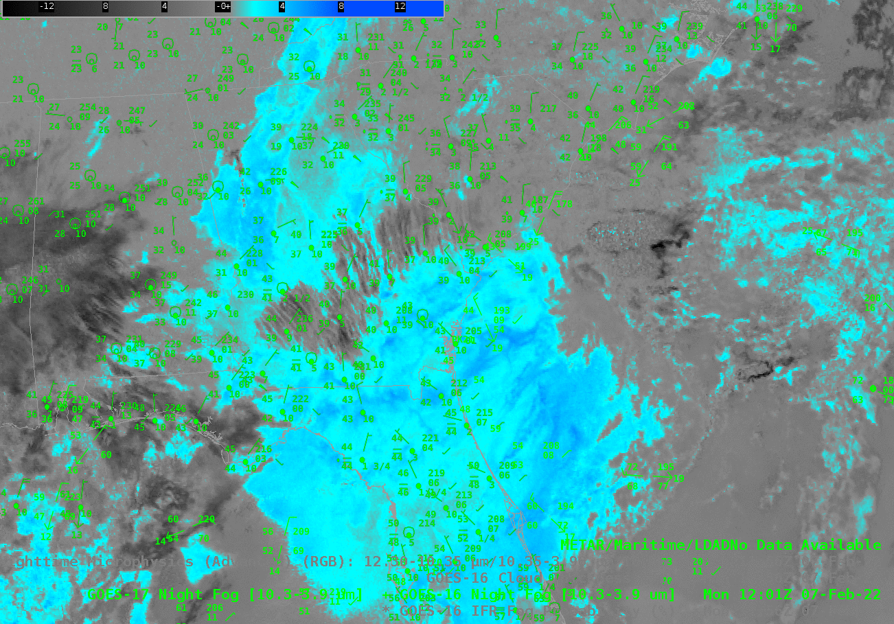
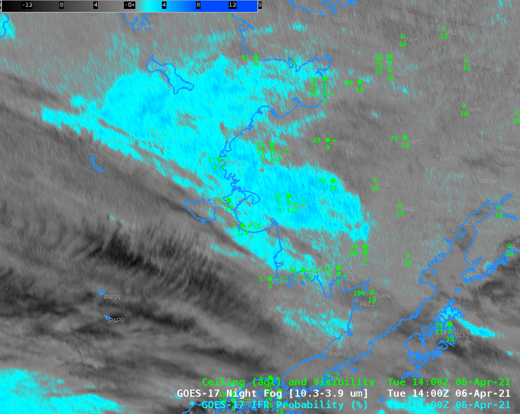
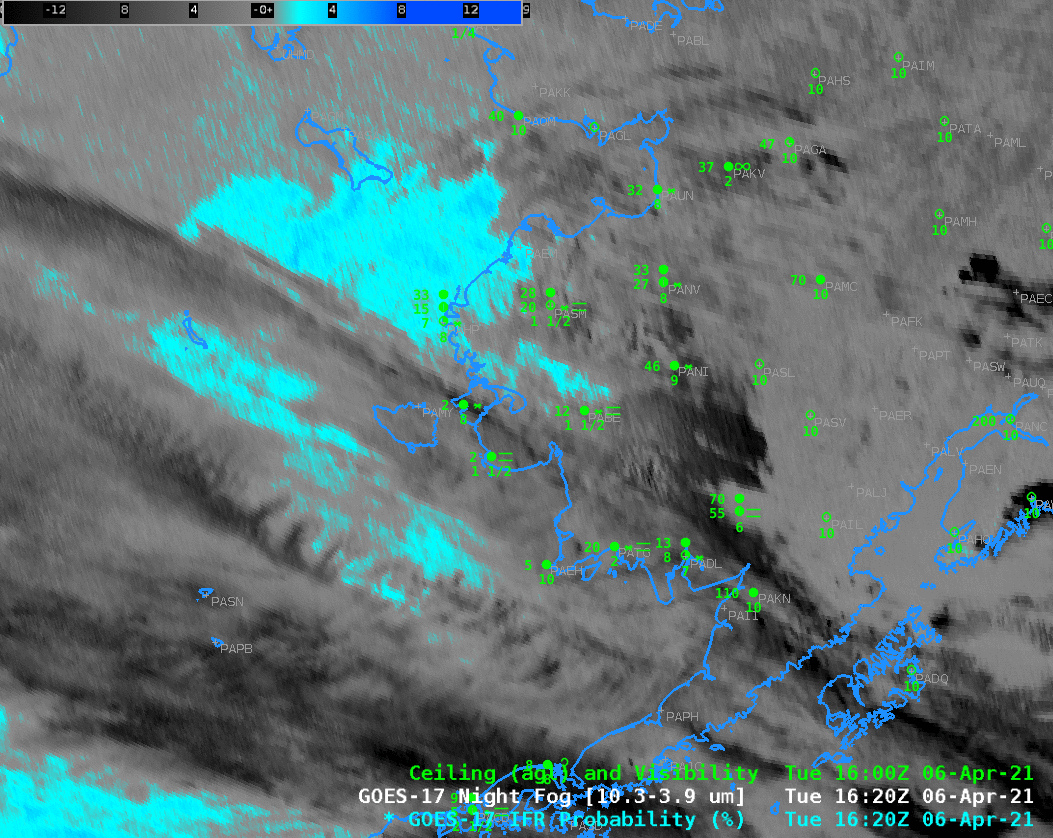
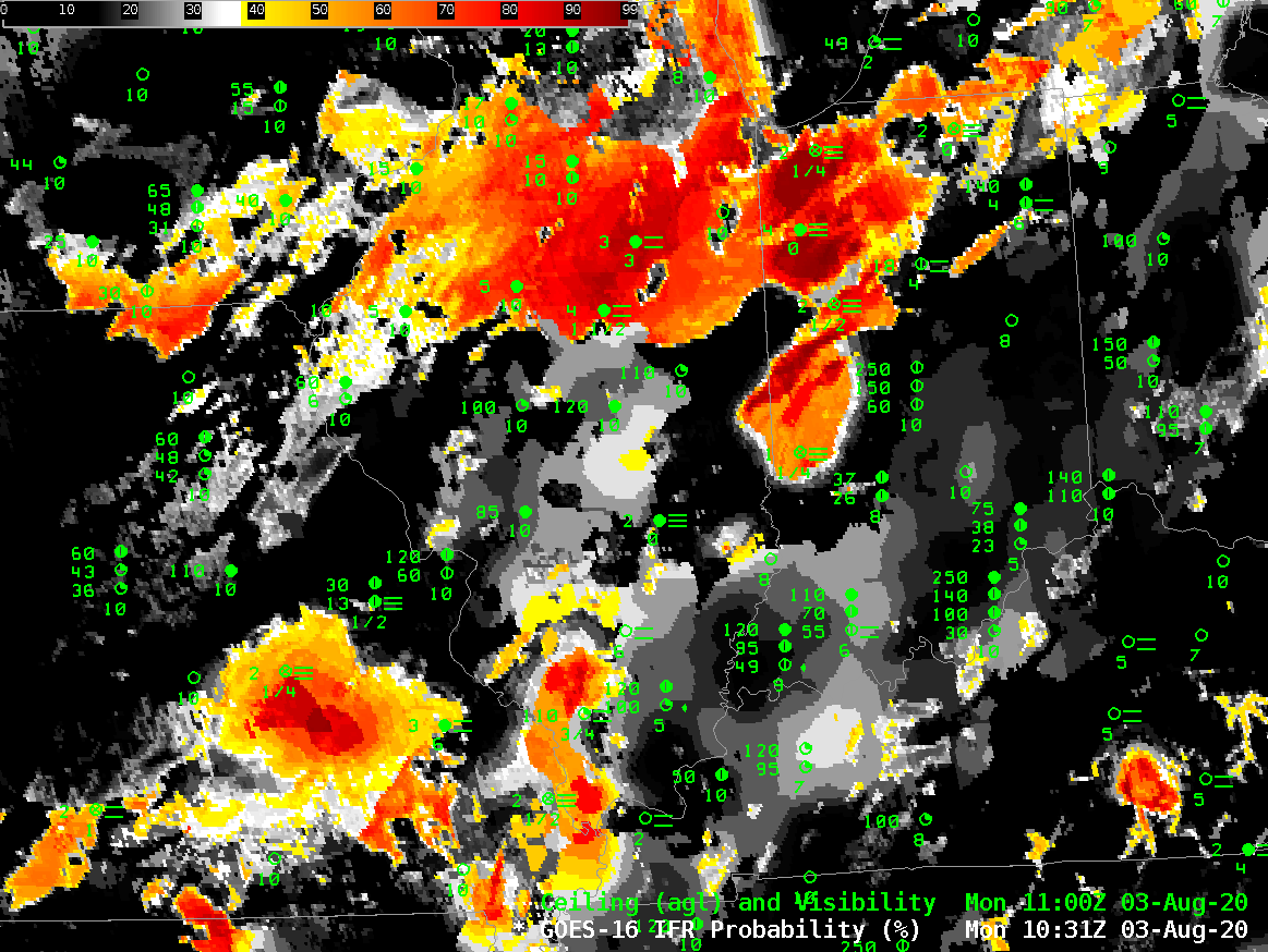
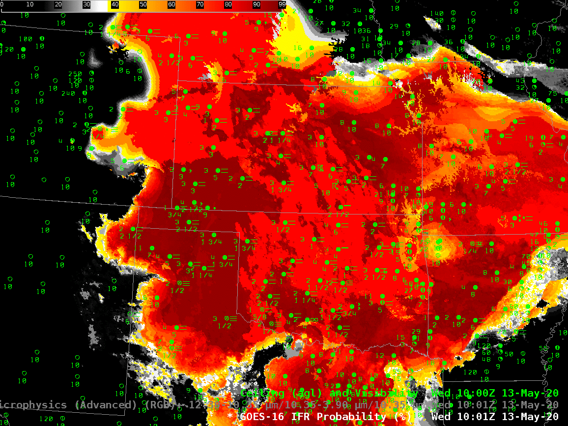
At 1156 UTC, a similar distribution to the three fields continues. Note how the presence of cirriform clouds over south-central Georgia affects the fields. The Night Fog BTD and Night Microphysics RGB both change radically, and IFR probabilities reduce — in part because the algorithm is less confident that low clouds exist. The small IFR Probabilities continue around Atlanta’s airline hub, important information from an aviation standpoint!

GOES-16 Night Fog Brightness Temperature Difference (10.3 µm – 3.9 µm), Night time microphysics RGB, and GOES-R IFR Probability, 1156 UTC on 7 February 2022 (Click to enlarge)

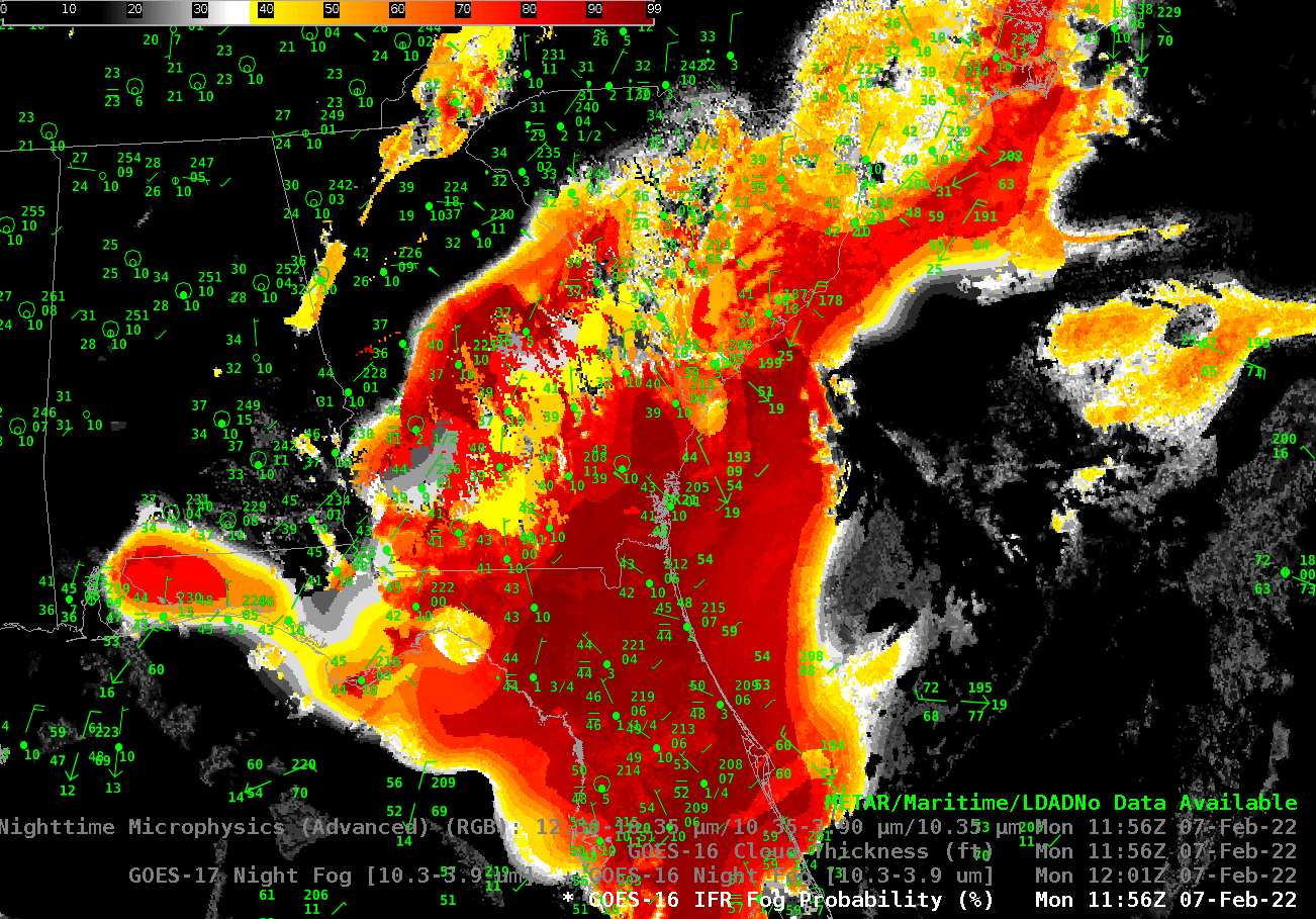
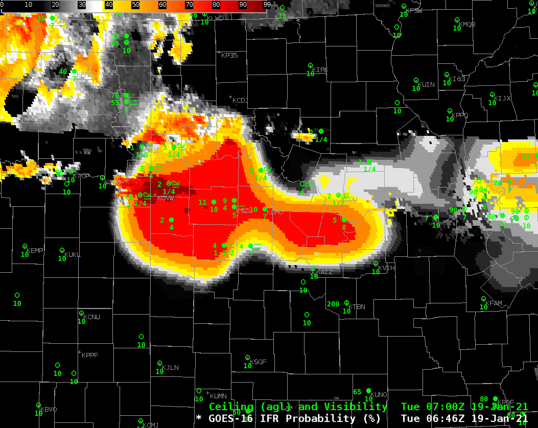
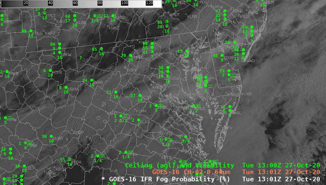
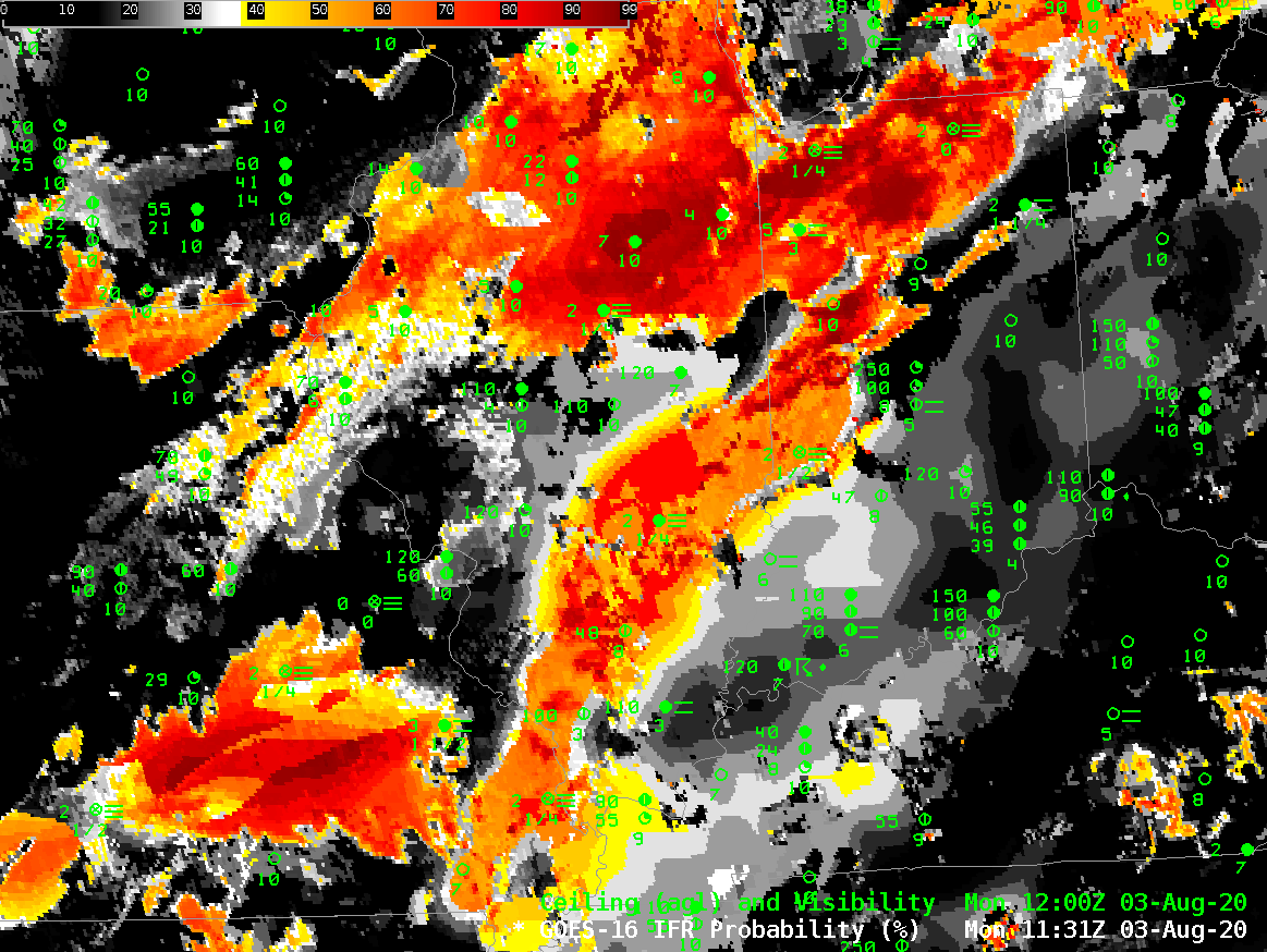
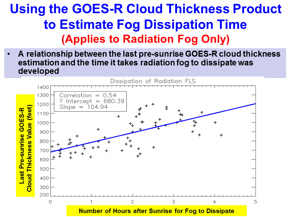
The toggle below compares IFR Probability with GOES-R Cloud Thickness. This is close to the time around sunrise/sunset when GOES-R Cloud Thickness are not computed because of quickly changing reflected solar shortwave infrared (3.9 µm) radiation; indeed, the cutoff can be viewed in the SSW-NNE terminator line over the Atlantic at the eastern edge of this image. If the low clouds on this day were strictly radiation (a dubious claim in the presence of rain!), then this scatterplot could be used to help decide when conditions might clear.

GOES-R IFR Probability and GOES-R Cloud Thickness fields, 1156 UTC on 7 February 2022 (Click to enlarge)

Fog backed up against the front range of the Rockies

GOES-16 Night Fog Brightness Temperature Difference (10.3 µm – 3.9 µm) and Nighttime microphysics RGB, 0901 UTC on 11 May 2021, along with observations of ceilings (AGL) and visibility

The toggle above compares Night Fog Brightness Temperature difference fields at 0901 UTC on 11 May over Colorado and surrounding states. Both fields can be used to identify regions of stratus/low stratus — and by inference, fog. At this time, however, it is a challenge to use these satellite-only products because of widespread mid/upper-level clouds over eastern Colorado, Kansas and Nebraska. Note how the blue/cyan regions in the Night Fog Brightness Temperature Difference field show through into the Nighttime Microphysics RGB; the green component of that RGB is the Night Fog Brightness Temperature Difference field.

On this day, the high clouds prevented the Brightness Temperature Difference alone from highlighting regions of fog. IFR Probability fields, below from the same time, show that this field better outlined the region of low clouds/fog over the High Plains. The field incorporates both Night Fog Brightness temperature difference fields — to determine where stratus clouds might be — and Rapid Refresh model estimates of low-level moisture — to determine where saturation might be occurring. Where the satellite detects stratus clouds, and where the Rapid Refresh model suggests low-level saturation, high IFR Probability (as over southeastern Colorado) results, in accordance with, on this day, observations. If high clouds are present (as over much of eastern Colorado), IFR Probability can still occur because the Rapid Refresh data shows low-level saturation. Note also that the extensive cloud cover over Kansas and Nebraska — elevated stratus — does not have a strong signal in the IFR Probability fields.

This product blends the strengths of satellite observations and the strength of model estimates.

GOES-16 Night Fog Brightness Temperature Difference  (10.3 µm – 3.9 µm) and IFR Probability, 0901 UTC on 11 May 2021, along with observations of ceilings (AGL) and visibility

IFR Probability fields over the Bering Sea

GOES-17 IFR Probability from 1220 – 1710 UTC on 6 April 2021 (Click to enlarge)

GOES-17 IFR Probability fields, above, show a large region of high probabilities to the south and west of Alaska over the Bering Sea. This region of low clouds is encroaching onto shore and demonstrates how the field could be used to predict the onset of lower ceilings. The Night Fog brightness temperature difference animation, below, spanning the same times, documents how high clouds can make mask the satellite detection of low clouds. The animation also shows how the signal changes when the Sun rises (mot noticeable after about 1600 UTC). The Night Fog Brightness Temperature difference field is a component of the Nighttime Microphysics RGB; if the Night Fog Brightness Temperature difference cannot detect low fog because of high clouds, then the Nighttime Microphysics RGB similarly will not detect low clouds.

GOES-17 Night Fog Brightness Temperature Difference (10.3 µm – 3.9 µm) fields, 1220 UTC – 1710 UTC on 6 April 2021 (click to enlarge).

The toggles below of Night Fog Brightness Temperature difference and GOES-17 IFR Probability at 1400 UTC (below) and 1620 UTC (bottom) underscore how the IFR Probability field can give useful information in regions underneath high clouds. If you were scheduled to be on a boat in the Bering Sea on this day, for example, would you expect any visibility?

Toggle between GOES-17 IFR Probability and GOES-17 Night Fog Brightness Temperature Difference (10.3 µm – 3.9 µm) fields, 1400 UTC on 6 April 2021 (click to enlarge). Surface observations of ceilings and visibilities at 1600 UTC are also plotted.
Toggle between GOES-17 IFR Probability and GOES-17 Night Fog Brightness Temperature Difference (10.3 µm – 3.9 µm) fields, 1620 UTC on 6 April 2021 (click to enlarge). Surface observations of ceilings and visibilities at 1600 UTC are also plotted.

The imagery below, from webcams at Togiak (at 1700 UTC) (source), show the low clouds along the coast.

Webcam image from Togiak AK, 1715 UTC 6 April 2021, looking north
Webcam image from Togiak AK, 1715 UTC 6 April 2021, looking west

Coastal fog under clouds in South Carolina

GOES-16 Brightness Temperature Difference (10.3 µm – 3.9 µm), 0831 – 1331 UTC 1 March 2021 (Click to enlarge)

GOES-16 Night Fog Brightness Temperature Difference (BTD) fields (10.3 µm – 3.9 µm), above, show different cloud types in and around South Carolina before and through sunrise on 1 March 2021. Before sunrises, low clouds — stratus and fog — are characterized by blue/cyan/aqua colors in this enhancement. The positive brightness temperature difference arises because of emissivity differences in small cloud droplets for shortwave (3.9 µm) and longwave (10.3 µm) infrared radiation. Negative brightness temperature differences occur for higher clouds.

The presence of high clouds interferes with the satellite’s ability to view low clouds. Although one can infer a low cloud’s presence from an animation (and the assumption that the cloud doesn’t substantively change when a high cloud overspreads it), it’s a bit more difficult to extrapolate the cloud base from the cloud top behavior. In other words: Are the low clouds highlighted actually fog? Note also how the BTD enhancement changes as reflected solar radiation around sunrise starts to overwhelm any differences attributable to emissivity.

IFR Probability fields, shown below, combine the strength of satellite detection of low clouds with the strength model depiction of low-level saturation. IFR Probabilities will be quite high where satellites detect low clouds, and where Rapid Refresh model simulations show near-surface saturation. But if high clouds are in the way, IFR Probabilities can still be large if the Rapid Refresh model shows low-level saturation. This is occurring off the coasts of South and North Carolina. Note also: IFR Probability fields aren’t changing radically as the sun rises.

GOES-16 IFR Probability, along with surface observations of ceilings and visibility, 0831 UTC – 1326 UTC 1 March 2021 (Click to enlarge)
Night Fog Brightness Temperature Difference, Night time microphysics RGB, GOES-16 IFR Probability, 1001 UTC on 1 March 2021 (Click to enlarge)

The toggle above compares the Night Fog BTD with the Night time microphysics RGB (an RGB that takes as its green component the Night Fog BTD), and the GOES-16 IFR Probability fields at 1001 UTC on 1 March, shortly before sunrise. There is an obvious relationship between the RGB color and the regions of low clouds highlighted in the BTD by blue/cyan/aqua colors; the color of the RGB is tempered by the cloud temperature, however: the blue component of the RGB is the longwave infrared brightness temperature, and that is different over the ocean compared to over southwestern Georgia (for example). Note also how IFR Probability shows large values under the deep clouds over northwest South Carolina/western North Carolina.

Why is fog occurring offshore? Moist air over South Carolina is moving over relatively cool shelf waters, and cooled to its dewpoint; advection fog is the result. The toggle below shows surface dewpoints in the low 60s over coastal South Carolina. Sea-surface temperatures, shown at bottom from VIIRS at 0700 UTC and GOES-16 at 1300 UTC, show cool shelf waters with surface temperatures in the 50s (F).

GOES-16 IFR Probability with surface observations of ceilings/observations and surface METARs, 1001 UTC on 1 March 2021 (Click to enlarge)
NOAA-20 ACSPO VIIRS Sea Surface Temperatures (0701 UTC) and GOES-16 SST Temperatures (1301 UTC), click to enlarge

IFR Probability over Missouri

GOES-16 IFR Probability, 0646 – 1501 UTC on 19 January 2021 (Click to enlarge)

GOES-16 IFR Probability fields, above, show a gradual expansion southward of the regions of highest probability of reduced visibility. As the fields encroach over stations, visibilities and ceilings are reduced: there is a very good relationship between observed IFR conditions and enhanced IFR Probabilities. This field could be used on 19 January to predict the onset of low ceilings and reduced visibilities.

You will note that there are hourly changes to the IFR Probability fields. Rapid Refresh model data used in the computation of IFR Probability is updated each hour when a more recent model simulation is incorporated into the data. You can also identify regions where satellite data are not used because high clouds are preventing a satellite view of low stratus: there are regions where IFR probability is an unpixelated mostly uniform field.

The Night Time microphysics RGB for the same period, shown below, also highlights the region of low clouds as a cyan/yellow feature slowly moving southward. In principle, this field is only showing you that stratus clouds are present, because information about the cloud base (supplied by the Rapid Refresh model in IFR Probability fields) is lacking.

The challenge of using the Night Time Microphysics field is also apparent near the end as the Sun rises and the color associated with the stratus clouds changes.

GOES-16 Night Time Microphysics RGB, 0646 – 1501 UTC, 19 January 2021 (Click to enlarge)

The toggle below compares the GOES-16 IFR Probability field and the GOES-16 Night Time Microsphysics RGB at 1201 UTC. A cirrus shield along the southern boundary of the IFR Probability field is hindering the ability of the Night Time Microphysics RGB there to detect low clouds.

GOES-R IFR Probability and Night Time Microphysics, 1201 UTC on 19 January 2021 (Click to enlarge)

Central Valley fog underneath high clouds

MIMIC Total Precipitable Water, 1300 UTC on 30 December 2020 (Click to enlarge)

A large storm moving ashore in British Columbia (0900 UTC Map), shown above in MIMIC Total Precipitable Water (from this site), was accompanied by widespread high clouds over much of the Pacific Coast of the United States. The 1511 UTC image, below, shows GOES-16 “clean window” (10.3 µm) infrared imagery, with high clouds apparent.

GOES-16 “Clean Window” infrared imagery (10.3 µm) at 1511 UTC on 30 December 2020

Satellite-only detection of fog/low clouds will be challenged on this day by the abundance of high clouds that block the satellite’s view of low stratus decks. Indeed, the ‘Night Fog’ brightness temperature difference field, below, allows for only periodic glimpses of what is happening near the surface. There are indications of fog — but it is challenging even in the animation to determine the horizontal extent of the fog regions.

GOES-16 ‘Night Fog’ Brightness Temperature Difference (BTD, 10.3 µm – 3.9 µm), 1111 – 1516 UTC on 30 December 2020, along with surface observations of ceilings and visibilities

GOES-16 Low IFR Probability fields, below (note: GOES-17 IFR Probability fields are still undergoing testing in preparation for their being deemed operational) highlight two regions of visibility restrictions: One is off the coast of central California, and a another is a narrow ribbon of reduced visibilities in the Central Valley. This case highlights a strength of IFR Probability fields: You get a useful and consistent signal even if high clouds are blocking the satellite view of low clouds. This is because Rapid Refresh Model estimates of low-level saturation are incorporated into the Probability fields.

GOES-16 Low IFR Probability fields, 1116 – 1511 UTC, 30 December 2020, along with surface observations of ceilings and visibilities (Click to enlarge)

IFR Conditions over Virginia

GOES-16 Night Fog Brightness Temperature Difference (10.3 µm – 3.9 µm) and IFR Probability at 0901 UTC, along with 0900 UTC plots of surface ceilings and visibility (Click to enlarge)

GOES-16 IFR Probability fields, above, from 0901 UTC on 27 October 2020 (in a toggle with the Night Fog Brightness Temperature Difference), outline two regions of likely IFR conditions over Virginia and surrounding states. Southern Virginia shows restricted conditions, as does the high terrain along the spine of the Appalachians, extending up to Johnstown PA. (Surface observations largely agree with IFR Probability fields: IFR Probability is high where ceilings are low and visibilities are restricted; IFR Probability is low in regions where IFR conditions are not occurring).

Night Fog Brightness Temperature Difference fields (10.3 µm – 3.9 µm), struggle to identify regions of IFR conditions — elevated stratus (over western Virginia and western Maryland, for example) has a similar signal to fog over southeastern Virginia. There are also regions of high clouds above the low stratus over Maryland and Virginia surrounding middle Chesapeake Bay. In such regions, high IFR Probability is being driven by Rapid Refresh model predictions of low-level saturation.


Visible imagery (0.64 µm) toggled with the IFR Probability fields at 1301 UTC, below, show how IFR Probability fields can better discriminate between stratus and fog than visible imagery alone.

GOES-16 Band 2 Visible (0.64 µm) and IFR Probability, 1301 UTC on 27 October 2020 (Click to enlarge)

Use IFR Probability fields to identify regions that have low ceilings and reduced visibilities when Visible imagery (in the day) and Night Fog Brightness Temperature difference (at night). During the day time, this can be achieved by displaying both images at once.

GOES-16 IFR Probability underneath the Visible (0.64 µm) imagery, 1301 UTC, 27 October 2020 (with a transparency alpha of 0.9 applied; click to enlarge)

IFR Probability as a Heads Up in Indiana

Because IFR Probability includes both model information on low-level saturation and satellite information on low-level clouds, it can give an advanced warning on the development of fog when high clouds — at might occur behind departing convection, for example — prevent the satellite from viewing the low cloud beneath high clouds.  Consider the animation below, that shows IFR Probability fields along with surface observations of ceilings and visibilities plotted so that regions with IFR conditions can be identified.  IFR probability fields develop over northwest Indiana over the course of the night, especially over extreme northern Indiana where the east-west Indiana Toll road sits.

GOES-R IFR Probability fields, along with observations of ceilings and visibility, 0051 – 1321 UTC (every 10 minutes) on 3 August 2020 (Click to enlarge)

Compare the IFR Probability fields above to the Night Fog Brightness Temperature Difference (10.3 µm – 3.9 µm) field below. The field below historically has been used at night to identify regions of low clouds/fog — regions that are cyan in the enhancement are low clouds, regions that are black are high clouds. As the sun rises, the Night Fog brightness temperature difference field will struggle to identify regions of low clouds (although a different enhacement can be used to highlight the low cloud regions after sunrise). The satellite is not able to view low clouds over northern Indiana until the high clouds move out. Thus, a distinct indication of low clouds over the Indiana Toll road lags the suggestion of low clouds given by IFR Probability fields.

GOES-16 ‘Night Fog’ Brightness Temperature Difference (10.3 µm – 3.9 µm), every ten minutes from 0051 to 1321 UTC, 3 August 2020 (click to enlarge)

Consider the toggle below of GOES-R IFR Probability, Night Fog Brightness Temperature Difference and the Nighttime Microphysics RGB at 0601 UTC on 3 August.. IFR Probability fields show a developing region of IFR conditions (in yellow) over extreme NW Indiana. The two satellite-only detectors show only a scant suggestiong that fog is present. (A similar scenario is occurring near the bootheel of Missouri)

GOES-R IFR Probability, Night Fog Brightness Temperature Difference (10.3 µm – 3.9 µm), and Nighttime Microphysics RGB, 0601 UTC on 3 August 2020 (Click to enlarge)

At 0901 UTC, below, all three indicators of low clouds are in better agreement over northwest Indiana (and over the Missouri Bootheel) as high clouds move from those areas.

GOES-R IFR Probability, Night Fog Brightness Temperature Difference (10.3 µm – 3.9 µm), and Nighttime Microphysics RGB, 0901 UTC on 3 August 2020 (Click to enlarge)

Fields at 0931 and 1001 UTC continue this trend of stronger signals in the regions initially highlighted at 0601 UTC by the IFR Probability fields.

GOES-R IFR Probability, Night Fog Brightness Temperature Difference (10.3 µm – 3.9 µm), and Nighttime Microphysics RGB, 1031 UTC on 3 August 2020 (Click to enlarge)

By 1131 UTC, below, increasing solar reflectance over the eastern part of the domain has changed the signal in both the Nighttime fog and Nighttime microphysics RGB over northern Indiana and Ohio. The GOES-R IFR Probability signal however is maintained.

GOES-R IFR Probability, Night Fog Brightness Temperature Difference (10.3 µm – 3.9 µm), and Nighttime Microphysics RGB, 1131 UTC on 3 August 2020 (Click to enlarge)

IFR conditions over the Great Plains

Surface Analysis at 0900 UTC on 13 May 2020

Much of the central Plains of the United States was under easterly flow during the night on 12-13 May 2020, as suggested by the surface analysis above. Strong High Pressure over the Great Lakes and lower pressures over the Rocky Mountains drove that upslope flow. Consequently, IFR conditions were common over much of the Plains, as shown below.

The animation, below, of IFR Probability (overlain with surface observations and ceilings and visibilities) shows high probabilities. There is good correlation between regions with High IFR Probabilities — red and orange — and regions with low ceilings and reduced visibilities. The highest probabilities, dark red in the enhancement, occur where satellite data shows low clouds and where model data shows low-level saturation. Note that there is a trend towards less satellite information in the IFR Probability field with time over central Oklahoma and south-central Kansas because of developing convection.

GOES-16 IFR Probability fields, 0800-1136 UTC on 13 May 2020

The night time microphysics RGB, shown below, is also used to detect regions of low clouds; they typically appear yellowish at this time of year. The challenge with the RGB use in highlighting IFR conditions is two-fold: high clouds will mask the low cloud signal (as in the case of developing convection over Oklahoma, or with cirrus over Colorado and Nebraska). The RGB can also struggle to differentiate between fog and low stratus. Note also in this animation how the effect of the rising sun becomes apparent at the end of the animation over the eastern third of the image.

Night time Microphysics RGB, 0801-1136 UTC on 13 May 2020

In the toggle below, the signal of low clouds in the RGB, yellow/cyan over the Texas panhandle (for example) has an echo in the IFR Probability field. In the absence of high clouds, both products will show regions of low clouds. The Night Time Microphysics RGB gives extra information about the cloud type in regions where high clouds are blocking the satellite view of low clouds (the purple region over Colorado/Nebraska and the reddish regions over Kansas and Oklahoma). In contrast, the IFR Probabilty field in those regions gives no information on the character of the higher cloud; the IFR Probability field in those regions is flat (i.e., not pixelated), the hallmark of IFR Probability that is derived chiefly from model fields, so all an analyst can tell is that a high cloud is present.

GOES-16 IFR Probability and Night Time Microphysics RGB, 1001 UTC on 13 May 2020

IFR Probability with a frontal passage over Pennsylvania

GOES-16 ABI Band 2 (0.64 µm) Visible Imagery, 1000-1700 UTC on 11 May 2020

Frontal passage with extratropical cyclones will frequently be accompanied by low ceilings and reduced visibilities, that is, IFR conditions. A loop of visible imagery, above, suggests a surface cyclone (surface analyses are shown below) but it is difficult to determine from the imagery where low ceilings and reduced visibilities are present. Continue reading