Category Archives: Day/Night Boundary

Maintaining a signal through sunrise

IFRProbability1045_1215_1300step

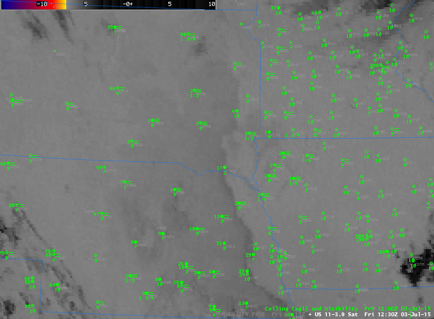
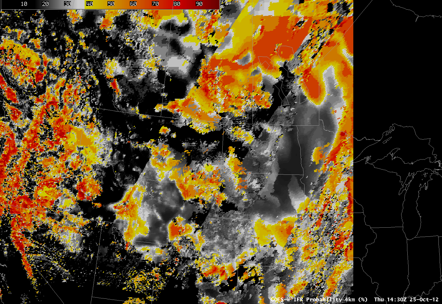
GOES-R IFR Probability fields, 1045, 1215 and 1300 UTC on 1 August 2016 (Click to enlarge)

A benefit of the GOES-R IFR Probability field is that a coherent signal is maintained through sunrise (or sunset). The traditional method of detecting fog that uses the brightness temperature difference between 10.7  µm and 3.9 µm cannot maintain a consistent signal through sunrise as the amount of reflected solar radiation with a wavelength of 3.9 µm increases, overwhelming the emissivity-driven differences between 10.7  µm and 3.9 µmbrightness temperatures that are observed at night. Consider the animation above, that shows GOES-R IFR Probability fields at 10:45 UTC, 12:15 UTC and 13:15 UTC. First: The GOES-R IFR Probability fields do a fine job of outlining where the lowest ceilings and poorest visibilities exist in this scene over Wisconsin both before sunrise and after.   The noticeable difference between the 1045 UTC and 1215 UTC fields is driven by a change in predictors that occurs as night transitions into day.

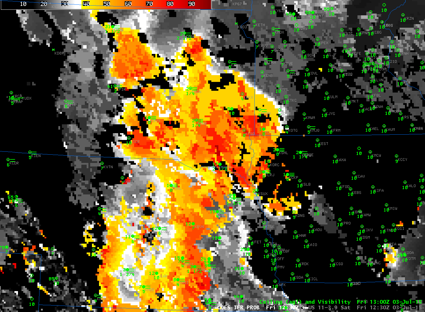
GOES-13 Brightness Temperature Difference fields (3.9 µm – 10.7 µm) are shown below. There is a strong signal at 1045 UTC, but little or no signal at 1215 UTC, before it returns (with opposite sign) at 1315 UTC.

BTD_01August2016_1045_1215_1315step

GOES-13 Brightness Temperature Difference Fields (3.9 µm – 10.7 µm) at 1045 UTC, 1215 UTC and 1315 UTC. (Click to enlarge)

Fog Detection at Sunrise

US_11-3.9_Sat_20150703_1230

Brightness Temperature Difference (10.7 µm – 3.9 µm) from GOES-13 at 1230 UTC, along with 1200 UTC Ceilings and Visibilities (Click to enlarge)

The Brightness Temperature Difference field is commonly used to detect low clouds in the atmosphere and to infer the presence of fog. At sunrise (and sunset), however, when the amount of reflected solar radiance with a wavelength of 3.9 µm is changing rapidly, features can be lost. For example, can you detect where the brightness temperature difference fields above relate to the observations of dense fog (Dense Fog Advisories were hoisted).

GOES-R IFR Probabilities are able to highlight regions of low clouds and fog through sunrise. The IFR Probability field for 1230 UTC on 3 July is shown below. It does a far better job of outlining the region of low clouds and fog.

GOES_IFR_PROB_20150703_1230

GOES-R IFR Probabilities computed from GOES-13 and Rapid Refresh model output, 1230 UTC 3 July 2015 (Click to enlarge)

Animations of the fields, of course, play to the strength of GOES-13 temporal resolution and aid detection. GOES-R IFR Probabilities and Brightness Temperature Difference Field animations are available.

Fog over Pennsylvania

GOES_IFR_PA_18August2014loop

GOES-R IFR Probabilities computed from GOES-13 data, hourly from 0500 through 1300 UTC 18 August 2014

River valley fog developed over Pennsylvania during the early morning hours of 18 August 2014, and the case is a good test of the GOES-R IFR Probability fields. IFR Probabilities are low at 0500 UTC (1 AM local time) and subsequently increase rapidly. In this case, the fields may be overpredicting where fog is present, as visible imagery just after sunrise suggest it was confined mostly to river valleys. In the animation above, the areal extent of the IFR Probabilities drops between 1100 UTC and 1215 UTC as the sun rises (the terminator is apparent in the 1100 UTC image, running from western Maryland north-northwestward to extreme western New York) and visible imagery can be used to more effectively cloud-clear the fields. A toggle between these two times is below. In this case, it is important to understand the geography underneath the IFR Probability field to hone the forecast.

GOES_IFR_PA_18August2014_1100-1215

GOES-R IFR Probabilities computed from GOES-13 data, at 1100 and 1215 UTC 18 August 2014

GOES13_BTD_18August2014loop

GOES-East Brightness Temperature Difference Fields (10.7µm – 3.9µm), hourly, from 0500-1100 UTC 18 August 2014

The Brightness Temperature Difference field, above, is the heritage method of detecting low stratus and inferring the presence of fog. Interpretation is complicated because high clouds (initially present over the southwestern portion of the scene, and moving eastward) prevent the satellite from viewing low clouds. In addition, as the sun rises (at the end of the animation, at 1100 UTC), solar radiation changes the character of the the brightness temperature difference field.

Data from the MODIS on board both Terra and Aqua can also be used to create both brightness temperature difference fields and IFR Probability fields. The toggle below, using ~0700 UTC data from GOES and from MODIS, shows the distinct advantage present in the MODIS field’s superior spatial resolution (1-km at sub-satellite point vs. 4-km at the sub-satellite point for GOES). River valleys are more evident in the MODIS data, by far, than in the GOES data.

GOES_MODIS_IFR_18August2014_07

GOES-R IFR Probabilities computed from GOES-13 data and from MODIS data, at 0700 UTC 18 August 2014

The Day-Night band on Suomi NPP at 0718 UTC showed that the densest fog was largely confined to river valleys.

SNPP_DNB_18August2014_0718UTC

Suomi NPP Day/Night Band, 0718 UTC on 18 August 2014

An animation of the fog burning off from GOES-14 (in special 1-minute SRSO-R scanning operations) is available here. It’s also on YouTube.

IFR Conditions on the West Coast as a front passes

GOES_IFR_PROB_20130930_loop

GOES-15-based GOES-R IFR Probabilities (Upper Left), GOES-15 Brightness Temperature Difference Product (10.7 – 3.9 ) (Upper Right), Color-shaded topographic map (Lower Left), GOES-15 Visible imagery and Suomi/NPP Day/Night Band (Lower Right), all times as indicated (click image to enlarge)

A strong low pressure system — the first strong system of the Fall Season — has made landfall along the Pacific Northwest Coast, and it provides an opportunity to see how GOES-R IFR Probabilities perform with extratropical systems.

Several aspects of the IFR Probability Fields — which are far more coherent than the Brightness Temperature Difference fields — require explanation. There is an increase in the IFR Probability off the coast of Oregon in the 4th image in the loop. This jump — from IFR Probabilities near 55% (orange) to Probabilities near 68% (darker red-orange) — is likely caused by a changed in the Rapid Refresh model output that is suggesting a greater likelihood of low-level saturation. Note that this region in the very next image displays the characteristic signature of the boundary between day-time predictors being used and night-time predictors being used (IFR Probabilities drop from orange yellow — 39%). In the early part of the animation, the IFR Probability field off the Oregon Coast maintains the flat (un-pixelated) look that is characteristic of a region where only Rapid Refresh model output is being used in the computation of IFR Probabilities because high cloud are present. GOES-R Cloud Thickness (of the highest water-phase cloud, not shown) would not be computed in this region, then, for two reasons: ice and mixed-phase clouds are present and it is during twilight conditions.

IFR and near-IFR Conditions are observed along the coast at Newport and North Bend before the frontal passage. IFR Probabilities are high along the coastal range, somewhat reduced in the Willamette Valley, high again in the Cascades, and lower again downstream of the Cascades. Note how the higher IFR Probabilities do take into account the presence of terrain; brightness temperature difference fields use only satellite data. Thus, after the frontal passage, when near-surface winds are west and south-west (that is, upslope), the IFR Probabilities remain high on the windward side of mountain slopes. (They are typically high, for example, at Sexton Summit — over KSXT — where IFR conditions are present until about 1100 UTC)

Suomi-NPP Day/Night band data can sometimes be used to discern regions of cloudiness. However, the Moon Phase is now a waning crescent that has not quite risen at the times shown in the animation above.

IFR Conditions over southwest mainland Alaska

Hourly GOES-R IFR Probability fields over southwest Alaska, 0500 to 1700 UTC 15 July 2013

The IFR Probability fields over southwest Alaska early on July 15 2013 show the influence of multiple cloud layers moving northward out of Bristol Bay and the Bering Sea starting near 0900 UTC.  IFR probabilities drop (because satellite data are not included as predictors when multiple cloud layers exist), and the field becomes flatter.  That is, it has less horizontal variability (especially compared to its pixelated nature when satellite data are included).  IFR conditions are largely confined to within the region of high IFR probabilities.

Two obvious boundaries are present in the field.  At 0800 UTC, a boundary extends southwest to northeast, with higher values to the north and west.  At 1500 UTC, a boundary extends southeast to northwest with higher values to the north and east.  In both cases, this line is the terminator, and daylight is occurring north of the line.  In general, IFR probabilities increase during the day (where they are diagnosed) because the cloud-clearing algorithm operates with a lot more certainty when visible imagery can be used to identify clouds.

MODIS data can be used in Alaska because Alaska’s high latitude ensures that MODIS overpasses are frequent (especially along the north slope of Alaska).  Three overpasses could be used between 0700 and 1415 UTC over this small region of southwest Alaska to give high-resolution depictions of IFR probabilities.  Using these high-resolution images with the high temporal resolution available from GOES-West gives a full description of the IFR Probability field over Alaska.  The 0832 UTC image suggests multiple cloud layers are still over Bristol Bay/the Bering Sea, and the 1415 UTC image shows both the day-night boundary and an IFR Probability field determined largely by model data.

MODIS-based GOES-R IFR Probabilities over southwest Alaska, 0654 UTC, 0832 UTC and 1415 UTC 15 July 2013

IFR Conditions over Georgia on a Summer Morning

Animation of GOES-East Water Vapor Imagery (6.7 µm), Brightness Temperature Difference Product (10.7 µm – 3.9 µm) and GOES-R IFR Probability computed with GOES-East data, 1000 UTC on 11 July 2013

The satellite animation, above, shows ample evidence of multi-layered clouds over Georgia and surrounding states, in a region where ceilings and visibilities approached/exceeded IFR conditions.  The traditional method of determining regions of fog/low stratus — the brightness temperature difference between the 10.7 µm and 3.9 µm channels — gives no information here because low clouds are screened by higher ice-phase clouds.

GOES-R IFR Probability fields merge information from GOES Imager data and the Rapid Refresh Model.  Even if GOES Imager data gives little information, GOES-R IFR Probability fields will give valuable information because they are also use information from the Rapid Refresh model.  Because the IFR Probability fields don’t include satellite data, probabilities are lower.  The large region of yellow — IFR Probabilities around 40% — sits over many stations that are reporting IFR conditions.   Note how IFR Probabilities are higher over North Carolina where satellite data are being used in the computation of the field — but there are fewer reports there of IFR conditions (despite the higher probability).  Temper the interpretation of the IFR Probabilities with knowledge of what is being used to compute them.

The evolution of IFR Probability fields can give a Head’s Up to deteriorating conditions in the atmosphere.  Note in the hourly animation below how probabilities initially do increase over regions that subsequently have IFR or near-IFR conditions.  At the end of the animation, there is an obvious boundary between different probabilities over northeast Georgia (Orange values around 55%) and western Georgia (values around 40%).  That southeast-to-northwest boundary shows where nighttime predictors are being used (to the west) vs. daytime predictors (to the east) in the computation of IFR Probabilities.

GOES-R IFR Probabilities (hourly) from 0200 through 1100 UTC, 11 July 2013

Lake Superior Plus High Dewpoints Means Fog

GOES-R IFR Probabilities computed from GOES-East, and surface observations of ceilings/visibilities (Upper Left), GOES-East Brightness Temperature Difference (10.7 µm – 3.9 µm) (Upper Right), GOES-R Cloud Thickness computed from GOES-East (Lower Left), GOES-R IFR Probabilities computed from MODIS (Lower Right)

The combination of cold Lake surface temperatures in the 40s and 50s over Lake Superior and mid-Summer dewpoints in the 60s to near 70 is a recipe for fog over the upper midwest. North winds behind a complex of thunderstorms fostered the development of fog and low stratus over the upper midwest early in the morning on July 8th, as shown in the imagery above.

The GOES-R IFR Probability fields seamlessly track the expansion of fog/low stratus in the region around western Lake Superior;  highest probabilities are confined to regions where IFR or near-IFR conditions are observed.  The IFR Probabilities also downplay regions where the brightness temperature difference field is showing a signal (northwest Minnesota) but where visibility obscurations are small.

IFR Probabilities are not as large over southern upper Michigan or over north-central Wisconsin, regions where multiple cloud layers mean that the satellite component does not contribute to IFR Probability computation, resulting in a smaller value.  Note that Cloud Thickness is not initially computed there either:  Cloud Thickness describes the thickness of the lowest water-based cloud layer in non-twilight conditions.  If there are multiple cloud layers that include mixed-phase of ice clouds, cloud thickness is not computed.  Note also that cloud thickness is not computed in the hours around sunrise (i.e., during twilight conditions).

By 1702 UTC, the final image, the Summer Sun has burned off much of the fog and low stratus, with the exception being along the shorline of Lake Superior.  MODIS-based IFR Probabilities have much sharper edges because of the higher resolution of the MODIS instrument compared to the GOES Imager.

Continuity through sunrise

GOES-R IFR Probabilities (Upper Left), computed from GOES-East, Brightness Temperature Difference (10.7 µm – 3.9 µm) computed from GOES-East, GOES-R Cloud Thickness (Lower left), Ceiling and Visibility observations (Lower right)

The animation of the GOES-R IFR Probability product, above, shows one of its strengths:  it has a similar look during night and day.  The traditional fog product created by the brightness temperature difference between 10.7 µm and 3.9 µm data from GOES-East, switches sign as the sun rises and the amount of reflected 3.9 µm radiation increases.  The IFR Probability maintains a steady signal that matches observed IFR conditions.

Note that the Brightness temperature difference product shows a signal along the Louisiana/Texas border (over the Toledo Bend Reservoir on the Sabine River), and also over Lake Sam Rayburn, Lake Livingston and Lake Conroe in east Texas.  It is possible that there is shallow fog over these bodies of water (post-sunrise imagery shows no signal);  the signal might also arise from the approximately 1-pixel co-registration error between the 3.9 µm and 10.7 µm channels on GOES-13. This possibly erroneous signal in the brightness temperature difference does propagate into the GOES-R IFR probability field.

Day/Night Transition artifacts

GOES-R IFR Probability, 1430 UTC on 25 October 2012

The predictors used by the GOES-R IFR Probability algorithms change as night turns to day and vice versa.  For example, the daytime predictors include the visible satellite imagery.  The change in predictors occurs when the solar zenith angle is less than 85 degrees (that is, when the sun is just rising). For solar angles between 85-90 degrees, temporal continuity has an increased importance and therefore the IFR probabilities look very similar to the previous temporal images.  When the solar zenith angle is between 80-85 degrees temporal metrics are used combined with current visible channel data (only if certain tests are passed that prove the data is of good quality). The cloud mask sometimes has difficulty detecting low clouds in this region so it still is not fully utilized until the solar zenith angle drops to below 80 degrees, where the cloud mask and the full array of daytime predictors are used. This leads to discernible changes in the probability fields, as shown above.  Two boundaries, extending southwest to northeast (roughly parallel to the terminator) are apparent, one from extreme northwest Utah through central Montana and into Canada (where the solar angle is around 85 degrees) and one from northwest Colorado through northwest South Dakota into Manitoba (where the solar angle increases above 80 degrees).   This transition zone is less noticeable in the Summer because of the Earth-Sun geometry.  It is very difficult to create the GOES-R Cloud Thickness product when the solar zenith angles are between 75-90 degrees so the product is currently not available in this region.  This is why the Cloud Thicknesses cut off over eastern Oregon and show back up over central Missouri.

GOES-R Cloud Thickness for 1430 UTC, 25 October 2012

GOES-R IFR Probability gives information in the day too!

GOES-R IFR Probability from GOES-East (Upper left), GOES-East Visible (Upper Right), GOES-R Cloud Thickness (Lower left) and GOES-East Brightness Temperature Difference (Lower Right)

The GOES-R IFR Probability serves a useful purpose in the day:  It highlights where, in a field of clouds, the lowest visibilities and ceilings are likely.  In the image above from coastal North and South Carolina and Georgia. cloudiness is hugging the coast, as indicated both in the visible and in the tradiational brightness temperature difference product.  Highest probabilities of IFR conditions are depicted near Statesboro and Savannah GA, where ceilings and visibilities are lowest.