Category Archives: Uncategorized

Fog over upstate New York and northern Pennsylvania

GOES-16 Band 2 Visible (0.64 µm) imagery, IFR Probability fields, GOES-R Cloud Thickness, 1411 UTC on 16 March 2022. Surface observations of ceilings and visibilities at 1400 UTC are also included. (Click to enlarge)

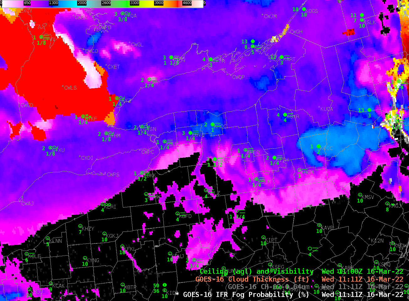
The toggle above shows early-morning (1411 UTC, i.e., 9:11 AM EDT) Fog in valleys over northern Pennsylvania and the southern tier of upstate New York. IFR Probability fields neatly overlap the regions of reduced ceilings and visibilities, with some exceptions in the narrow river valleys where visible imagery (with 0.5-km resolution at nadir) can easily resolve tendrils of fog; infrared data (with nadir resolution of 2 km) used by IFR Probability struggles to identify fog in those regions. The thickest fog is indicated over Lake Ontario.

Cloud Thickness fields can be used to estimate when fog will dissipate. If you observe the last image before sunrise (Cloud Thickness is not computed for a time period when the sun rises — or sets — because of rapid changes in the reflected component of shortwave infrared — 3.9 µm — solar radiation). Note in the image the diagnosed thinness to the fog over the river valleys. You might expect that fog to dissipate first. Cloud Thickness is not computed in regions of multiple cloud layers, such as, in this case, southwestern Ontario, where only the IFR Probability field is shown.

GOES-16 IFR Probability and Cloud Thickness, 1111 UTC on 16 March 2022, along with observations of ceiling heights and visibilities (Click to enlarge)

What did things look like at 1700 UTC, after the daily rise in temperature had caused substantial erosion of fog? The image below shows fog persisting over Lake Ontario, where IFR Probabilities are uniformly high. IFR conditions persist north of the lake but the southern shore of Lake Ontario shows less obstruction; one might (correctly!) infer southerly winds over the region. Indeed, Rochester and Buffalo both show southerly winds and dewpoints near 40. Toronto on the north shore of Lake Ontario has light southeast winds and fog at this time. There is a noteworthy east-west boundary in IFR Probability to the south of Wiarton, Ontario (METAR CYVV with 2-mile visibility and a 3500-foot ceilings, the station just south of the Bruce Peninsula). Careful inspection of the visible imagery there reveals an east-west cirrus cloud, so that IFR Probability is being computed mostly with output from the Rapid Refresh model there; the model is indicating low-level saturation so IFR Probabilities are large. Just to the south, clouds are not indicated, so IFR Probabilities are small.

GOES-16 Band 2 Visible (0.64 µm) imagery and IFR Probability fields, 1701 UTC on 16 March 2022. Surface observations of ceilings and visibilities at 1700 UTC are also included. (Click to enlarge)

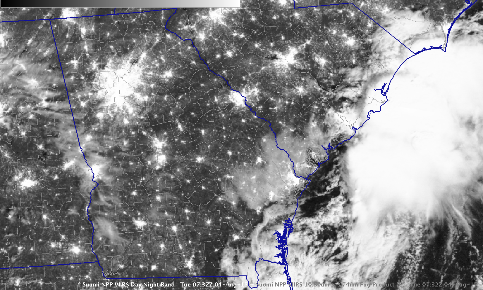
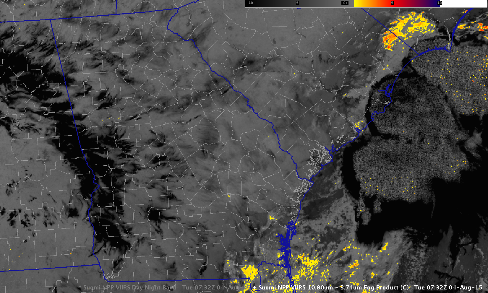
There are many ways to detect low clouds/fog day and night. In this case, a lack of high clouds over Pennsylvania meant that the Night Microphysics RGB gave a good signal where stratus clouds were present. IFR Probability allows for a consistent signal from night into day — and it includes a consistent signal where high clouds prevent the Night Microphysics RGB from indicating low clouds (Click here to see a toggle between the Night Microphysics RGB and GOES-R IFR Probability (with surface observations) at 1111 UTC).

Low Stratus under Cirrus

GOES-16 ‘Night Fog’ Brightness Temperature Difference (10.3 µm – 3.9 µm), 1151 and 1246 UTC on 9 October 2020 (Click to enlarge)

The extensive cirrus shield from Hurricane Delta in the Gulf of Mexico made difficult the satellite-based detection of stratus and low clouds over much of the Deep South on Friday 9 October. The Night Fog Brightness Temperature Difference is also affected by increased solar reflectivity at 1246 UTC in the imagery above. The low clouds over southern Illinois are no longer detected, for example, and the high cirrus of Delta becomes much darker — in both cases because of increased reflectivity of 3.9 µm solar radiation.

The toggle below between the Night Fog Brightness tempreature difference and the Band 4 near-infrared “Cirrus” channel just after sunrise (1246 UTC) shows the extensive cirrus signal in both images. Widespread cirrus is not uncommon, thus the difficulty in detection is not uncommon

GOES-16 Night Fog Brightness Temperature Difference (10.3 µm – 3.9 µm) and near-infrared 1.38 µm “Cirrus” Band 4, 1246 UTC on 9 OCtober 2020 (Click to enlarge)

GOES-R IFR Probability fields, below, compared to the Night Fog Brightness Temperature fields highlight how IFR Probability, which fields include information about low-level saturation in the Rapid Refresh model, capably fills in regions of fog/low stratus underneath high clouds. It is useful for situational awareness in fog detection when satellite imagery is showing only upper-level clouds. For example, note the large values of IFR Probability in western Kentucky, under the high cirrus, or in northeast Texas! There is good spatial correlation between high IFR Probabilities and reduced ceilings/visibilities. The correlation between the Night Fog Brightness Temperature difference field and reduced ceilings/visibilities is smaller because of low visibility under cirrus (as occurring over northwestern TN and much of LA, for example). Note that IFR Probability fields also give information where IFR conditions are not occurring under cirrus: central Mississippi, for example.

GOES-16 IFR Probability and Night Fog Brightness Temperature Difference (10.3 µm – 3.9 µm) at 1151 UTC on 9 October 2020 (Click to enlarge)

IFR Probability fields through sunrise (below) show a consistent signal, in part because of the Rapid Refresh model information on saturation.

GOES-16 IFR Probability fields, 1151 and 1246 UTC on 9 October 2020 (Click to enlarge)

The CIMSS-driven LDM feed that has supplied GOES-16 IFR Probability fields (and before GOES-R’s launch, GOES-13 and GOES-15 IFR Probability fields) to NWS offices will be terminated on or about 20 October. Operational creation of GOES-16 IFR Probability fields has shifted to NOAA/NESDIS, and the fields are now sent over the SBN to forecast offices. TOWR-S Build 19 is required to access and display these fields in AWIPS.

Fog over western Kansas

GOES-16 Low-IFR Probability, 0846 to 1341 UTC on 14 August 2020 (Click to enlarge)

Fog developed over western Kansas during the early morning of 14 August 2020 (helped along by above-normal precipitation in the past 30 days — shown here in an image created at this website). Low IFR Probability fields, above, show greatest probabilities of low ceilings and visibility restrictions in regions where they were observed: over western Kansas, with a sharp cut-off at the Colorado/Kansas border, and over western Oklahoma and the north Texas panhandle.

Compare the evolution of the Low IFR Probability field, above, to the evolution of the Night Fog brightness temperature difference (10.3 µm – 3.9 µm) field below.

The Night Fog field, below, has a region of strong return over western Kansas, but also two regions of weaker signals over central Kansas (where low clouds/fog are observed; note the regions in the brightness temperature difference field where the signal is very small, small grey pockets within the cyan, corresponding to the locations of towns in central Kansas) and over eastern Colorado (where low clouds/fog are not observed). Low IFR Probability fields are able to distinguish between the central Kansas and eastern Colorado because model predictions of low-level saturation are used to modulate the satellite-based signal: Low IFR Probability values are very small over Colorado (where the Rapid Refresh model is not predicting low-level saturation); values are larger over Kansas where ceiling and visibility reductions are occurring and where the Rapid Refresh model is suggesting low-level saturation is present). The brightness temperature difference field in Colorado might be driven by dry soils rather than low clouds. A brightness temperature difference signal can emerge at night because of soil emissivity differences (as noted earlier in this blog here).
Low IFR Probability fields are augmented underneath the convection that is apparent in the brightness temperature difference field over northwestern Arkansas. Satellite detection through the deep convection of low stratus in this region is impossible; the signal is driven by low-level saturation predicted by the Rapid Refresh model output.
As the sun rises, the brightness temperature difference field loses obvious cloud-detection signal because increasing amounts of reflected solar radiation (at 3.9 µm) overwhelm the emissivity-driven difference over low clouds at 3.9 µm and 10.3 µm. At some point after sunrise, the brightness temperature difference flips sign (and appears dark in the enhancement) because there is far more reflected solar radiation at 3.9 µm than at 10.3 µm.
The Low IFR Probability field by design includes temporal continuity around sunrise and sunset. This is most noticeable over central Kansas. The terminator sweep is noticeable in the field, but the values change only slowly in the hour surrounding the terminator. This temporal continuity is necessary because of the quick changes in detected 3.9 µm radiation that are occurring as solar reflectance changes occur.

GOES-16 Night Fog Brightness Temperature Difference (10.3 µm – 3.9 µm). 0846 to 1341 UTC on 14 August 2020 (Click to enlarge)

The relationship between MVFR Probability, IFR Probability and Low IFR Probability

GOES-16 MVFR Probability, IFR Probability and Low IFR Probability, 1136 UTC on 14 August 2020 (Click to enlarge)

Most of the posts on this blog discuss IFR Probability: The probability that IFR conditions are occurring. IFR, or Instrument Flight Rules conditions are defined as ceilings between 1000 and 3000 feet and/or visibilities between 1 and 3 miles. Two other Probability fields are created: MVFR Probabilities (MVFR, or Marginal Visual Flight Rules, are defined as ceilings between 3000 and 5000 feet and/or visibilities between 3 and 5 statute miles) and Low IFR Probabilities (LIFR, ceilings below 1000 feet and/or visibilities less than 1 mile). The animation above steps through the three fields from one time: MVFR Probability, IFR Probability and Low IFR Probability. As might be expected, MVFR Probability > IFR Probability > LIFR Probability.

Cursor readouts in AWIPS imagery are shown below; LIFR Probability fields are shown with the other two Probability fields are loaded underneath. The cursor readout (for the point just north and west of the upper left corner of the readout values) shows the relationship between the three fields. Low IFR Probability is shown in coral, IFR Probability in green, MVFR Probability in white. MVFR Probability values > IFR Probabilty values > LIFR Probability values.

GOES-16 Low IFR Probability with cursor readout of Low IFR Probability, IFR Probability and MVFR Probability, 1136 UTC 14 April 2020 (Click to enlarge)

Dense Fog over the central Mississippi River Valley

GOES-16 Brightness Temperature Difference field (10.3 µm – 3.9 µm) from 0417 to 1357 UTC on 28 August 2017 (Click to animate)

GOES-16 data posted on this page are preliminary, non-operational and are undergoing testing.

GOES-16 Brightness Temperature Difference fields (10.3 µm – 3.9 µm), above, show the development of stratus clouds (made up of water droplets) over the Plains during the morning of 28 August 2017. The Brightness Temperature for 10.3 µm is warmer than that for 3.9 µm during the night because cloud water droplets do not emit 3.9 µm radiation as a blackbody but those same cloud water droplets do emit 10.3 µm radiation more nearly as a blackbody would. The conversion from sensed radiation to brightness temperature does assume blackbody emissions; thus, the 3.9 µm brightness temperature is cooler where clouds made up of small water droplets exist. The animation above shows stratus clouds developing over Missouri and adjacent states. Dense Fog Advisories were issued near sunrise for much of the region (see image at bottom of this blog post) and IFR Conditions were widespread.

The animation above shows a positive signal over the western High Plains from Kansas northward to North Dakota. (Click here for the view at 1132 UTC on 28 August).

GOES-R IFR Probabilities are computed using Legacy GOES (GOES-13 and GOES-15) and Rapid Refresh model information; GOES-16 data will be incorporated into the IFR Probability algorithm in late 2017

How did GOES-R IFR Probability fields capture this event? The animation showing the fields every 30 minutes from 0215 through 1345 UTC on 28 August 2017, below, shows the development of High Probabilities in the region where Dense Fog was observed. There is a signal along the western High Plains, but it has low Probability; a conclusion might be that thin stratus has developed but that the Rapid Refresh model does not suggest that widespread low-level saturation is occurring. As the sun rises, the signal over the western High Plains disappears. Click here for a toggle between the GOES-R IFR Probability and the GOES-16 Brightness Temperature Difference field at 1115 UTC.

GOES-R IFR Probability fields, 0215-1345 UTC, 28 August 2017 (Click to enlarge)

Screen Capture of http://www.weather.gov at 1300 UTC on 28 August 2017 (Click to enlarge)

GOES-16 Data are Flowing

GOES-R IFR Probability that uses present GOES (GOES-13 and GOES-15) data in the computation of GOES-R IFR Probability fields was designed in anticipation of GOES-16 data that are now flowing to National Weather Service Forecast offices. Click here for a description of the Brightness Temperature Difference field values that are available now in AWIPS from GOES-16.

GOES-R FLS products are currently derived from GOES-13 and GOES-15 data. A GOES-16 version of the GOES-R FLS products will not be available until later in 2017.

Dense Fog over the Carolinas

GOES-13 Brightness Temperature Difference (3.9 µm – 10.7 µm), GOES-R IFR Probability and GOES-R Cloud Thickness at 1115 UTC on 17 January 2017 (Click the enlarge)

Dense Fog Advisories (National Weather Service Website) and IFR SIGMETs (Aviation Weather website) were issued early in the morning for dense fog over the southeastern United States. The toggle above from 1115 UTC on 17 January shows the Brightness Temperature Difference field (3.9 µm – 10.7 µm), the GOES-R IFR Probability Field, and the GOES-R Cloud Thickness fields associated with this dense fog event. Note the presence of high clouds over northern South Carolina and western North Carolina — the dark region in the Brightness Temperature Difference enhancement — prevents the brightness temperature difference field from highlighting that region of reduced ceilings/visibilities. The GOES-R Cloud Thickness field is not computed under cirrus either, as it relates 3.9 µm emissivity of water-based clouds to cloud thickness (based on a look-up table generated using data from a SODAR off the West Coast of the United States). If cirrus blocks the view, then, neither the Brightness Temperature Difference field nor the GOES-R Cloud Thickness field can give useful information about low clouds.

In contrast, the GOES-R IFR Probability field does give useful information in regions where cirrus clouds (and low clouds/fog) are present — because Rapid Refresh information about the lower troposphere can be used. IFR Probability values will be smaller in those regions because satellite predictors are unavailable, and the Probability incorporates both predictors from satellites and from Rapid Refresh model output — if the satellite predictors are missing because of cirrus, the IFR Probability values will be affected. Despite the smaller values, however, the IFR Probability fields in regions of cirrus are giving useful information for this event.

GOES-R Cloud thickness fields can be used to estimate Fog dissipation using the last GOES-R Cloud Thickness field produced before twilight conditions at sunrise (shown below for this case). (GOES-R Cloud Thickness is not computed during twilight conditions because of rapidly changing 3.9 µm emissivity related to the reflected solar radiation as the sun rises, or as it sets). This scatterplot gives the relationship between thickness and dissipation time after the Cloud Thickness time stamp (1215 UTC in this case). In this case, the thickest fog is near Athens GA; the algorithm predicts that clearing should happen there last, at about 1515 UTC.

GOES-R Cloud Thickness, 1215 UTC on 17 January 2017 (Click to enlarge)

Dense Fog in South Carolina and Georgia

Screenshot from Charleston WFO, 1230 UTC 4 August 2015

GOES-R IFR Probability fields computed from GOES-13 and Rapid Refresh Data, hourly from 0400 through 1215 UTC 4 August 2015 (Click to enlarge)

Dense fog developed over the piedmont of South Carolina/Georgia on 4 August 2015 in the wake of departing convection. The GOES-R IFR Probability fields, shown above hourly from 0400 to 1215, do parallel the development of the reduced ceilings and visibilities. Brightness Temperature Difference fields, below, from 0615 to 1215 UTC, do not show a strong fog signal until after 0800 UTC, yet IFR conditions at that time stretch from Walterboro SC (KRBW) southeastward to Eastman GA (KEZM) and Baxley GA (KBHC). GOES-R IFR Probabilities therefore give a better head’s up to a forecaster tasked with monitoring ceilings and visibilities.

Suomi NPP overflew the Southeast United States at ~0730 UTC on 4 August. Ample illumination from the waning three-quarter moon showed cloudiness over southeastern coastal South Carolina and adjacent parts of Georgia but the brightness temperature difference field does not suggest that these are all water-based clouds (such clouds generally fall in the yellow or orange part of the enhancement).

Suomi NPP Day Night Band visible (0.70 µm) image, 0732 UTC 04 August 2015 (click to enlarge)

Suomi NPP Brightness temperature Difference field (11.45 µm – 3.74 µm), 0732 UTC on 4 August 2015 (click to enlarge)

MODIS data from Terra and Aqua satellites can also be used to compute GOES-R IFR Probability fields, and two MODIS swaths were produced over South Carolina/Georgia early on August 4. Toggles between the 0337 Terra-based GOES-R IFR Probability Field and the 0755 UTC Aqua-based GOES-R IFR Probability fields are below. The larger values from MODIS — especially at 0755 UTC — suggest the fog was initially at small-scale horizontally. The 1-km resolution pixels from MODIS better capture any small-scale features.

MODIS-based (Terra) and GOES-based (GOES-13) GOES-R IFR Probability fields at ~0340 UTC on 04 August 2015 (click to enlarge)

MODIS-based (Aqua) and GOES-based (GOES-13) GOES-R IFR Probability fields at ~0800 UTC on 04 August 2015 (click to enlarge)

Post-thunderstorm Fog over Mississippi

GOES-R IFR Probability Fields, ~hourly, from 0300 through 1200 UTC on 19 May 2015 (Click to enlarge)

Thunderstorms moved through Mississippi (See this animation — from this Blog Post — of SRSO-R 1-minute imagery from 18 May), and the low-level moisture left behind allowed Dense Fog to form, and Dense Fog advisories were issued.

Multiple cloud decks — shown in the toggle, below, of Suomi NPP Day Night Band and Brightness Temperature Difference (11.45 µm – 3.74 µm) — prevented the traditional brightness temperature difference product from providing useful information. GOES-R IFR Probabilities, shown ~hourly in an animation above do highlight the region of developing IFR conditions. Low ceilings and reduced visibilities are commonplace in regions where IFR Probabilities are increasing over night. The predictors that are included to compute the IFR Probabilities are mostly model-based because of the multiple cloud layers that are present, and the IFR Probability field is somewhat flat as a result. Note that GOES-R IFR probabilities increase at the very end of the animation; when daytime predictors are used, probabilities are a bit higher than when nighttime predictors are used.

Suomi NPP Day Night Band visible imagery and Brightness Temperature Difference (11.45 µm – 3.74 µm) at 0818 UTC, 19 May 2015 (Click to enlarge)

Short Training Video

The video below is a short (11-minute) description of IFR Probability.

Alternatively, click the Link.

GOES-R Fog Product Examples

Fog detection fusing GOES, Terra/Aqua or Suomi/NPP Satellite data with Model output