Monthly Archives: June 2013

Fog detection in the land of the Midnight Sun

Brightness Temperature Difference (10.7 µm- 3.9 µm) from GOES-West (quarter-hourly timestep)

As above, but with a color enhancement applied (hourly timestep)

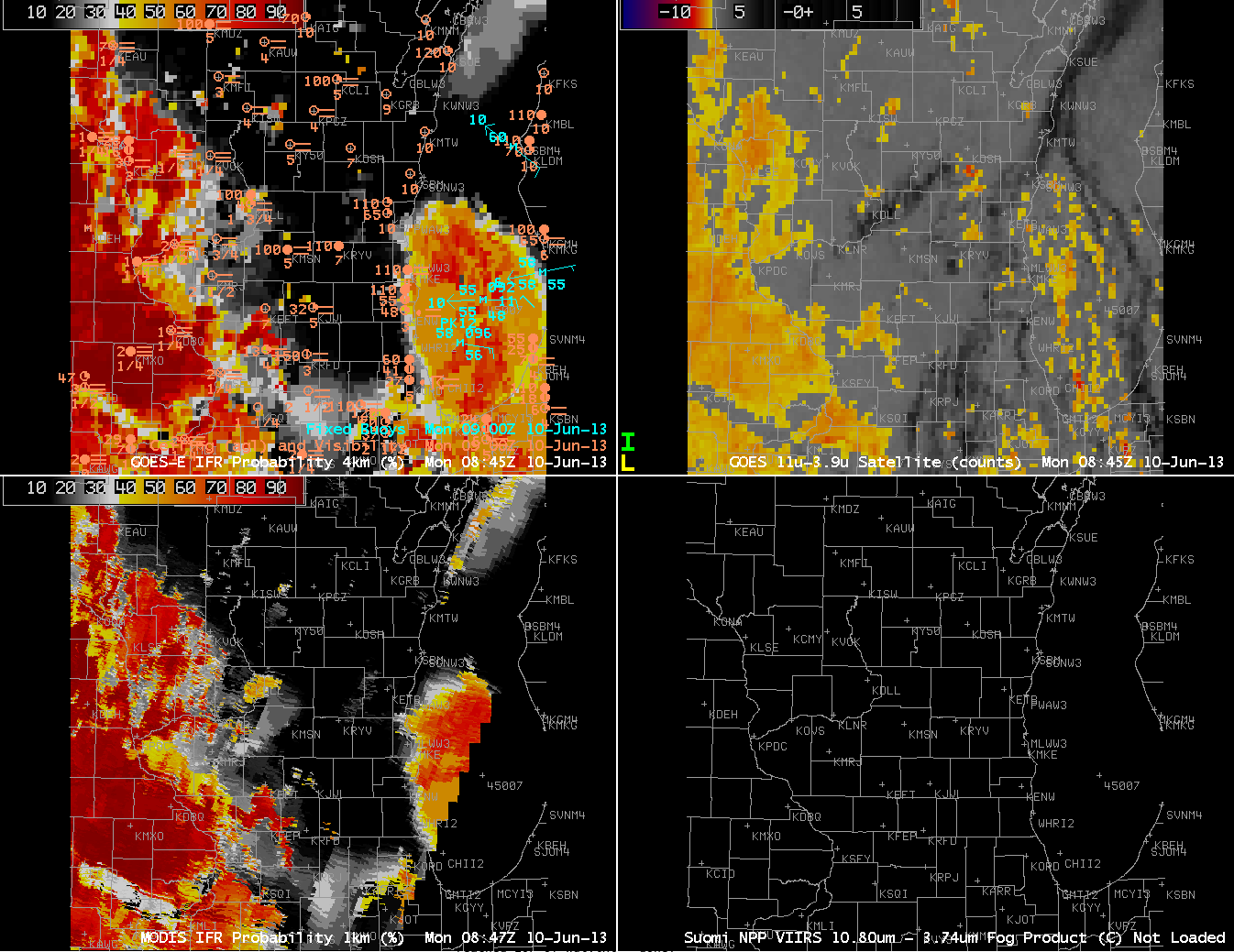
Over the continental United States, the brightness temperature difference can be used, sometimes, to approximate where fog and low clouds are present because water-based clouds (such as fog and stratus) have different emissivity properties for radiation at 10.7 µm and 3.9 µm.  In regions where the sun shines constantly, however, the brightness temperature difference product is harder to interpret because the abundance of scattered or reflected solar radiation with wavelengths near 3.9 µm.  In the examples above, the darker region (top animation) or lighter region (bottom animation) are regions of low clouds.  Regions of visibility obstruction — station PABA, for example (Barter Island on the shore of the Arctic Ocean) do not appear to be near fog/low stratus as indicated by the brightness temperature difference.

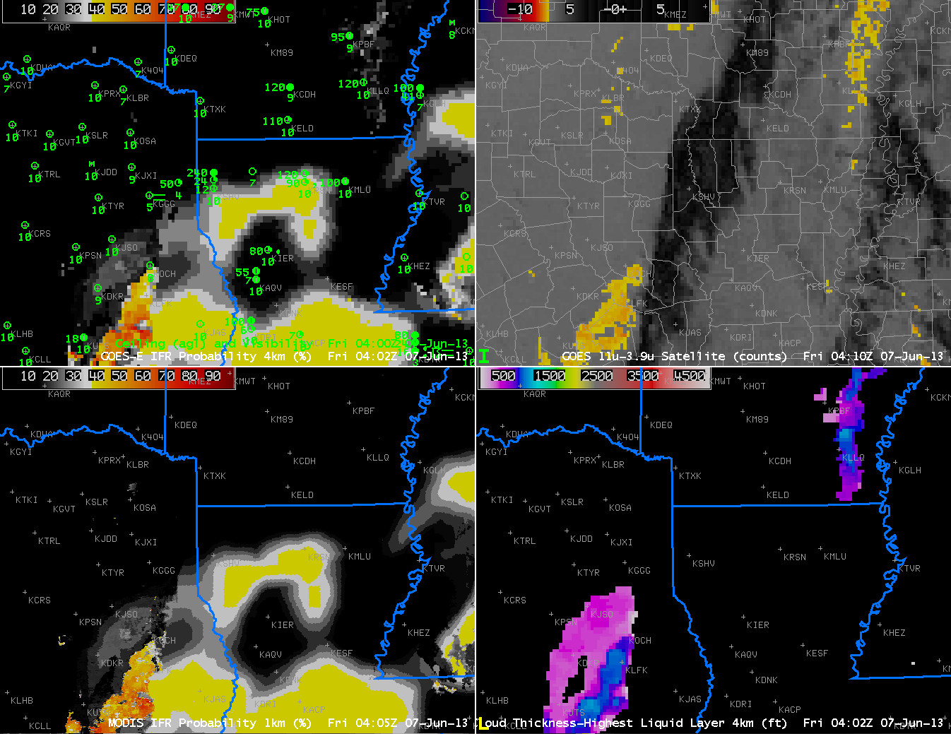
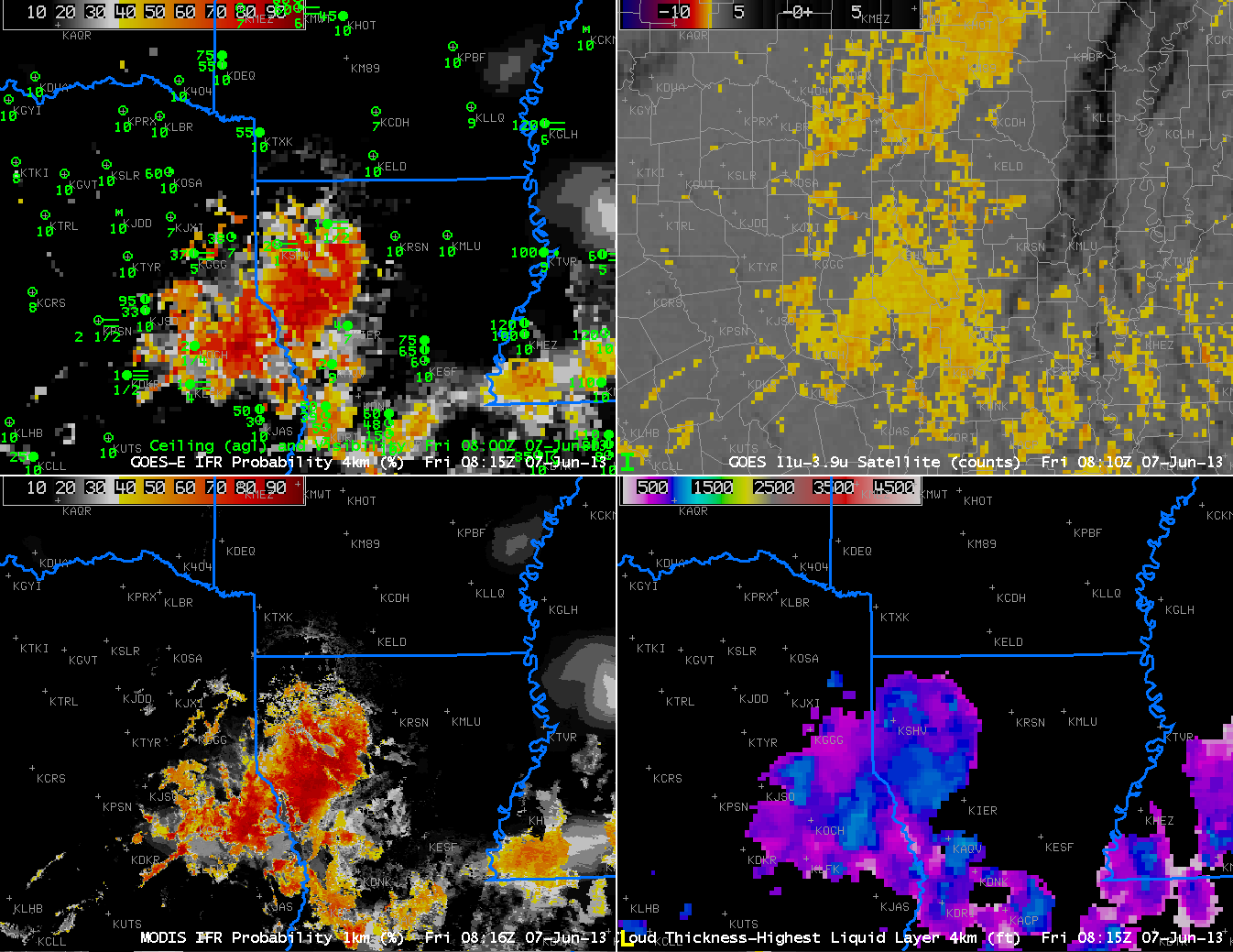
The GOES-R IFR Probability field combines Rapid Refresh data and GOES-West brightness temperature difference information (and other information, such as a cloud mask) to more accurately portray the horizontal extent of visibility obstructions.  The animation below suggests high probability of IFR conditions along the Arctic Ocean shore in northern Alaska.

There are regions at present over Alaska of significant visibility obstructions due to smoke.  These visibility obstructions are not predicted by the GOES-R Fog/Low Stratus product.  Smoke detection typically incorporates a brightness temperature difference between 10.7 µm and 12.0 µm, and the GOES-15 Imager does not include 12.0 µm detection.

GOES-R IFR Probabilities computed from GOES-West, along with surface ceilings and visibilities.  Times as indicated.

A visible image of the north slope of Alaska, below, shows fog and low clouds very near the Arctic shore.

GOES-15 Visible Imagery, 1700 UTC 28 June 2013

IFR Probability Fields capture back-door cold front in New England

Visible imagery around 0000 UTC on 27 June 2013 showing the slow advance of a backdoor coldfront over eastern New England.  The yellow arrows at the end highlight the front over New Hampshire.

A back-door coldfront moved westward through New England late in the day on June 26th, bringing with it cooler air and lowered ceilings.  How well did the IFR Probability field capture the low ceilings that came with the cooler air?

GOES-R IFR Probability fields computed from GOES-East, hourly from 2345 UTC on 26 June to 0445 UTC on 27 June.

Intially (2345 UTC), high probabilities of IFR conditions were limited to the cold waters east of New England. This is reasonable given the high dewpoints (upper 60s Fahrenheit) that prevailed New England on the 26th.  Light westerly winds would move that moist air over the cold Gulf of Maine, and advection fog would form.  As the backdoor front moved across the region, IFR probabilities increased as visibilities declined.  The animation of the IFR probability fields captures the leading edge of the maritime air.

Resolution: GOES vs. MODIS and Suomi/NPP over Appalachia

Brightness Temperature Difference (11µm – 3.74µm) at 0621 and 0750 UTC on 20 June 2013.  Data from VIIRS instrument on Suomi/NPP
Brightness Temperature Difference (10.7 µm – 3.9 µm) at 0625 and 0755 UTC on 20 June 2013.  Data from Imager GOES-East.

The GOES Imager, with a nominal (sub-satellite point) resolution of 4 km, has trouble detecting fog when that fog forms over very narrow valleys, as are common over the central Appalachians of the eastern United States.  Compare the views from the GOES Imager (the bottom images) to the view from the Suomi/NPP VIIRS instrument that has 1-km resolution.  VIIRS is much better able to capture the dendritic nature of valley fog, and also to detect it at all when the horizontal scale is very small (for example, the southwest-to-northeast oriented valleys in extreme southwest Virginia).  Thus, a signal will appear first in the high-resolution 1-km polar orbiter data, sometimes several hours before it appears in the coarser-resolution GOES Imager data.

These resolution issues that are apparent in the Brightness Temperature Difference fields, above, the traditional method of detecting fog and low stratus, carry over to the GOES-R IFR Probability fields.  Imagery below, from 0745 UTC on 20 June 2013 suggests that the higher-resolution MODIS data better captures the structure of fog in mountain valleys.  Note also the horizontal shift in the field that occurs because of the GOES parallax shift.

GOES-R IFR Probability fields computed from GOES-East and from Aqua MODIS data, 0745 UTC on 20 June 2013

Fog/Low Stratus over southern California viewed by many Satellites

Suomi-NPP VIIRS imagery at 0857 UTC 17 June 2013.  Imagery includes the Day/Night band (including regions north of Southern California within the Stray Light zone) and the brightness temperature difference between 11 µm and 3.74 µm

There are a variety of ways to detect fog and low stratus using satellites.  The imagery above uses VIIRS data aboard the Suomi/NPP satellite.  Both the Day/Night band and the brightness temperature difference product show a region of clear skies west of the Channel Islands, with low clouds hugging the coast from Los Angeles southward.  There are also low cloud signals in the brightness temperature difference field over the deserts of California, Arizona and Mexico.

MODIS-based imagery at 0853 UTC 17 June 2013.  The brightness temperature difference (10.8 µm – 3.9 µm ) and MODIS-based GOES-R IFR Probabilities

MODIS data also hints at a clear pocket west of the Channel Islands, and shows fog/stratus extending southward from Los Angeles along the coast.  Whereas the brightness temperature difference also shows a signal over the deserts of California, Arizona and Mexico, the GOES-R IFR probability field suggests probabilities for IFR conditions are enhanced only along the north coast of the Gulf of California.  The other signals over land are likely related to emissivity property differences in the dry soils over the deserts.  MODIS data does show the sharp edge to the fog/low stratus deck that has moved onshore over coastal northern Baja California.  That sharp edge demonstrates an advantage of 1-km MODIS data.

GOES-West Brightness Temperature Difference (10.7 µm – 3.9 µm ) and GOES-R IFR Probabilities computed from GOES-West data, 0900 UTC 17 June 2013

GOES-West data also suggest a clear spot west of the Channel Islands, with fog and low stratus that extends southward along the coast from Los Angeles.  The brightness temperature difference signal over the deserts of the southwest is not in the IFR probability field because the Rapid Refresh model data does not show low-level saturation (save for that small region along the north coast of the Gulf of California).  The cloud edge along the Pacific Coast is not quite so sharp as it is in the MODIS data because the pixel size of GOES is larger.  GOES data does have an advantage over MODIS, however:  it views the scene every 15 minutes so temporal changes can be monitored.

Lake Michigan Fog

Fog from Lake Michigan is a year-round hazard for travel in eastern Wisconsin.  One of the biggest crashes on an interstate in Wisconsin occurred in October 2002 on I-43 near Sheboygan as fog moved onshore.  Ten died in that event that included 25 vehicles.

Rain overnight followed by partial clearing led to widespread fog over the upper Midwest on June 10, 2013, and the IFR Probability products described the horizontal extent of the lowest visibilities.  Those low visibilities hugged the coast of Lake Michigan in eastern Wisconsin.

GOES-R IFR Probabilities, 0402 – 1345 UTC on 10 June 2013, computed from GOES-East

GOES-R IFR probabilities increase in two regions overnight:  over Iowa and in the western Wisconsin River Valleys, and over Lake Michigan.  Reduced visibilities are reported in and around Lake Michigan, and as the tweet up top shows, dense fog was reported along highways as well.  Water temperatures in the upper 40s over central Lake Michigan promote the development of fog, as dewpoints over Wisconsin were near 60.

GOES-R IFR Probabilities computed from GOES-East (Upper Left) and from MODIS (Lower Left);  GOES-East Brightness Temperature Difference Product (Upper Right), all from approximately 0845 UTC on 10 June 2013

The GOES Imager usually cannot resolve small river valleys.  Polar-orbiting data, however, usually can.  The MODIS-based IFR probability from 0847 UTC better resolves the Wisconsin River Valley over southwest Wisconsin, for example.

Low clouds over Louisiana

GOES-R IFR Probabilities computed from GOES-East (Upper Left), GOES-East Brightness Temperature Difference (Upper Right), GOES-R IFR Probabilities computed from MODIS data (Lower Left), GOES-R Cloud Thickness computed from GOES-East (Lower Right), every half hour from 0015 UTC to 1615 UTC on June 7 2013

GOES-R IFR Probabilities are shown for northwest Louisiana and surrounding states.  At the beginning of the animation, GOES-R fields are mostly model-based over much of Louisiana — the north-south oriented edge of high clouds is plain in the brightness temperature difference field starting around 0315 UTC, and the GOES-R IFR Probability field over Louisiana has the characteristic flat look of a field produced from mostly model (Rapid Refresh) data.  Note also that the Cloud Thickness product is not shown when high clouds are present.  It is computed only for low clouds in non-twilight conditions.

As the high and mid-level clouds move to the east, two things happen to the GOES-R fields. One, the Cloud Thickness field starts to show values.  And second, the GOES-R IFR Probability field starts to acquire the pixelated character that is common when satellite data are part of the field.

The are of high IFR probabilities is smaller than the region of enhanced brightness temperature difference, which at 0900 UTC covers much of Louisiana and Arkansas.  Over Arkansas, however, model data are de-emphasizing the possibility of reduced surface visibilities.  The low clouds there are stratus, off the ground, not fog.  Thus the IFR probability field gives a more accurate representation of where visibility restrictions at the surface are possible.  This is an important consideration in aviation forecasting.

As above, but for 0400 UTC (top) and 0815 UTC (bottom)

IFR Probabilities computed from MODIS data (lower left) show very similar areal coverage compared to the GOES-Based IFR probability fields, but small-scale variations in the field are much more evident, as should be expected given the difference in pixel footprint between the two satellites.

Advection fog over the Northeast as a front moves through

GOES-R IFR Probabilities, hourly, from 0500 UTC through 2002 UTC 3 June 2012

A cold front moving through eastern New England has drawn 60-degree dewpoints into that region of the country.  When that moist air then moves over the cold shelf waters and cold waters of the Gulf of Maine, fog and low stratus develop.  The GOES-R IFR Probability Field ably captures the regions of restricted visibility over coastal and offshore New England.  It also depicts the sharp northern edge of the restricted visibilities over Connecticut and Rhode Island.  The IFR probability field in the animation above is derived mostly from model data;  this is evident from the smooth nature of the field.  There are regions that are more pixelated within the smooth field.  These are regions where holes in the high cloud field associated with the front allow the satellite to see low water-based clouds.