 |
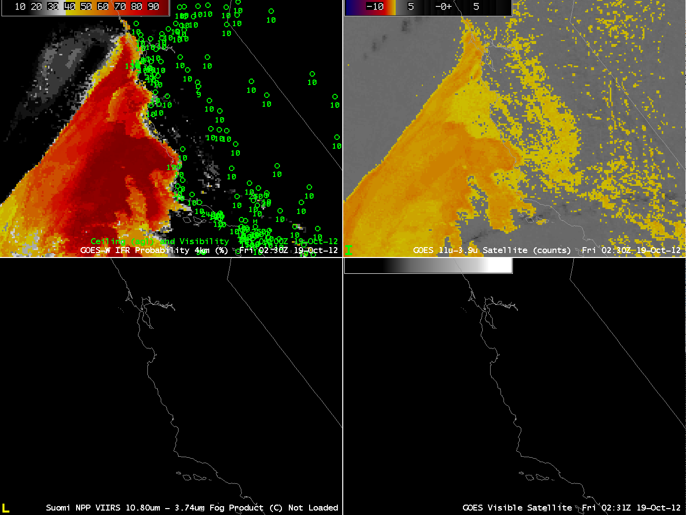
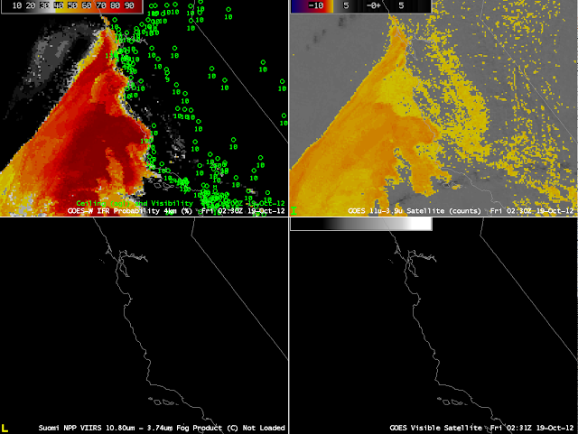
| GOES-R IFR Probabilities (Upper left) and GOES-15 brightness temperature difference (10.7 µm – 3.9 µm) (upper right) from 0200 UTC |
GOES-R IFR Probabilities can be used to evaluate and monitor the evolution of marine stratus as it (nightly) moves inland from the Pacific Ocean to adjacent land over California, as well as the evolution of fog and low clouds/haze over the central Valley of California. At 0200 UTC — near sunset — as shown above, IFR conditions are diagnosed from fused satellite and model data to be most likely offshore, despite a brightness temperature difference signal in California’s Central Valley, where airports are not reporting IFR conditions. In other words, the GOES-R IFR algorithm is correctly suppressing the satellite signal inland.
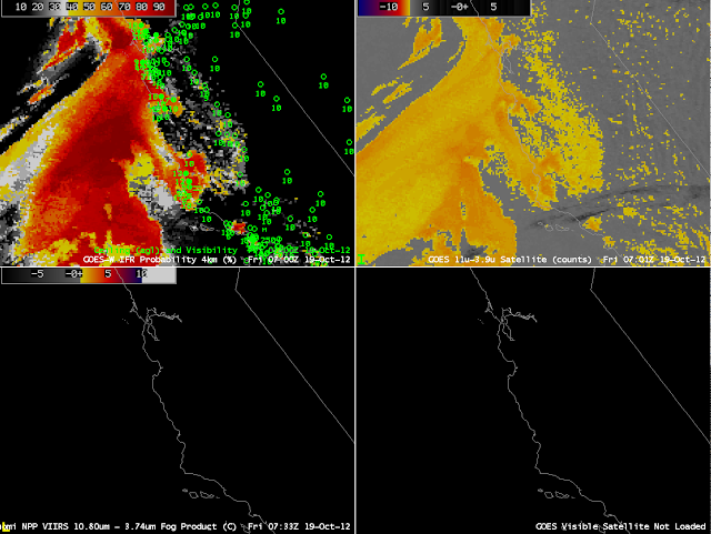 |
| GOES-R IFR Probabilities (Upper left) and GOES-15 brightness temperature difference (10.7 µm – 3.9 µm) (upper right) from 0700 UTC |
By 0700 UTC, ceilings and visibilities in the Salinas and Central Valleys have started to lower as IFR probabilities decrease.
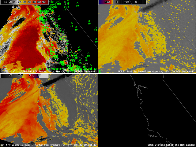 |
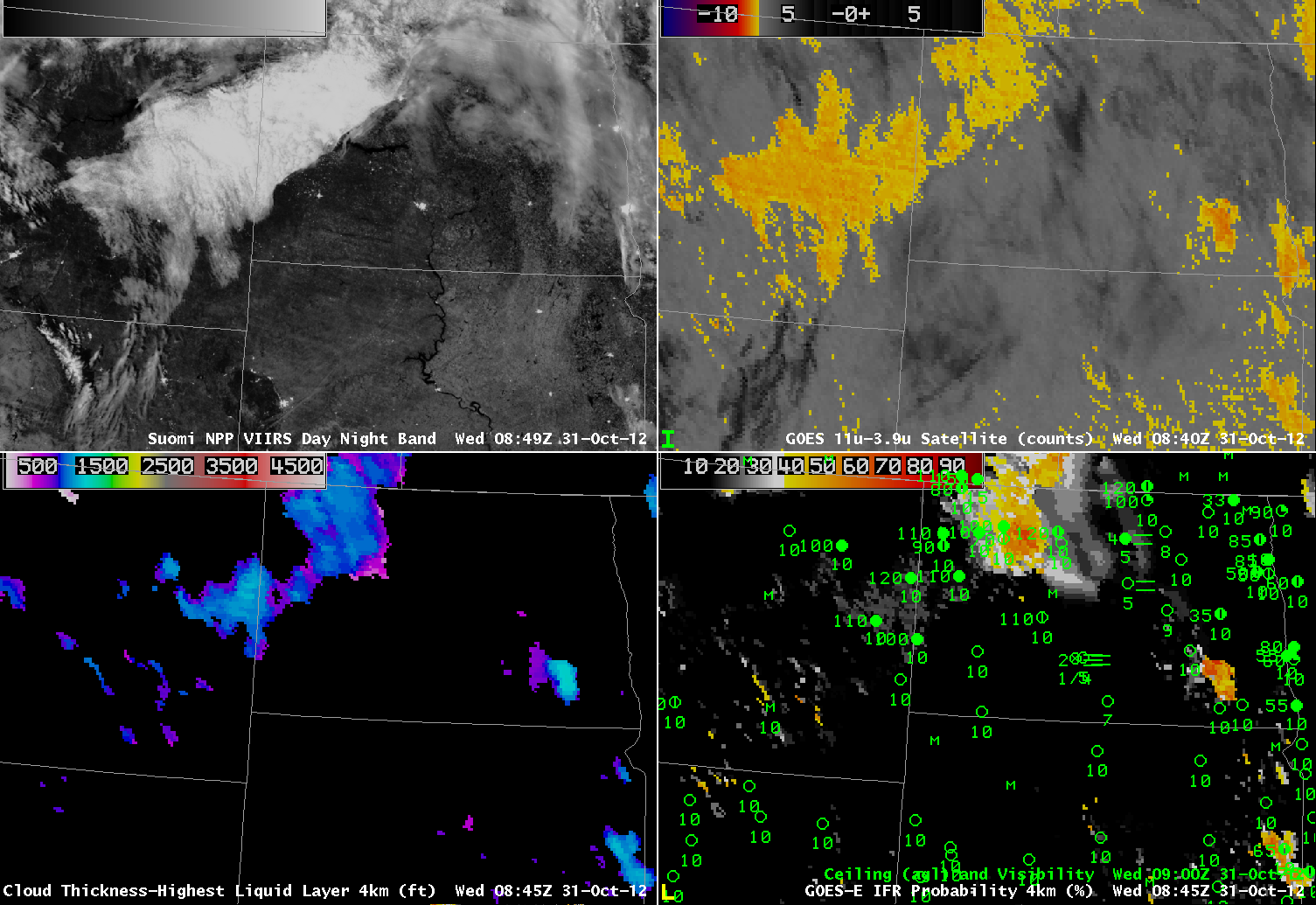
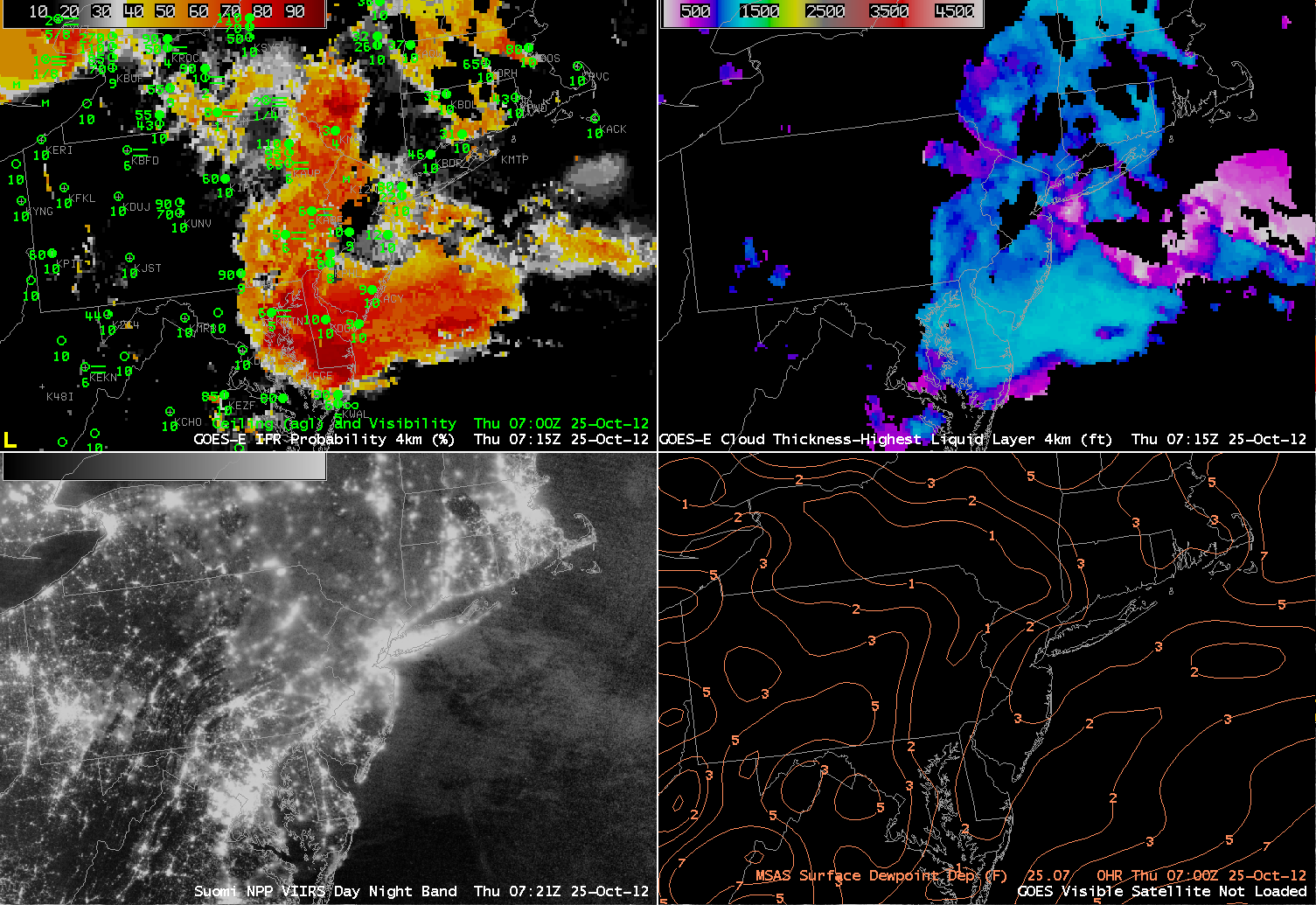
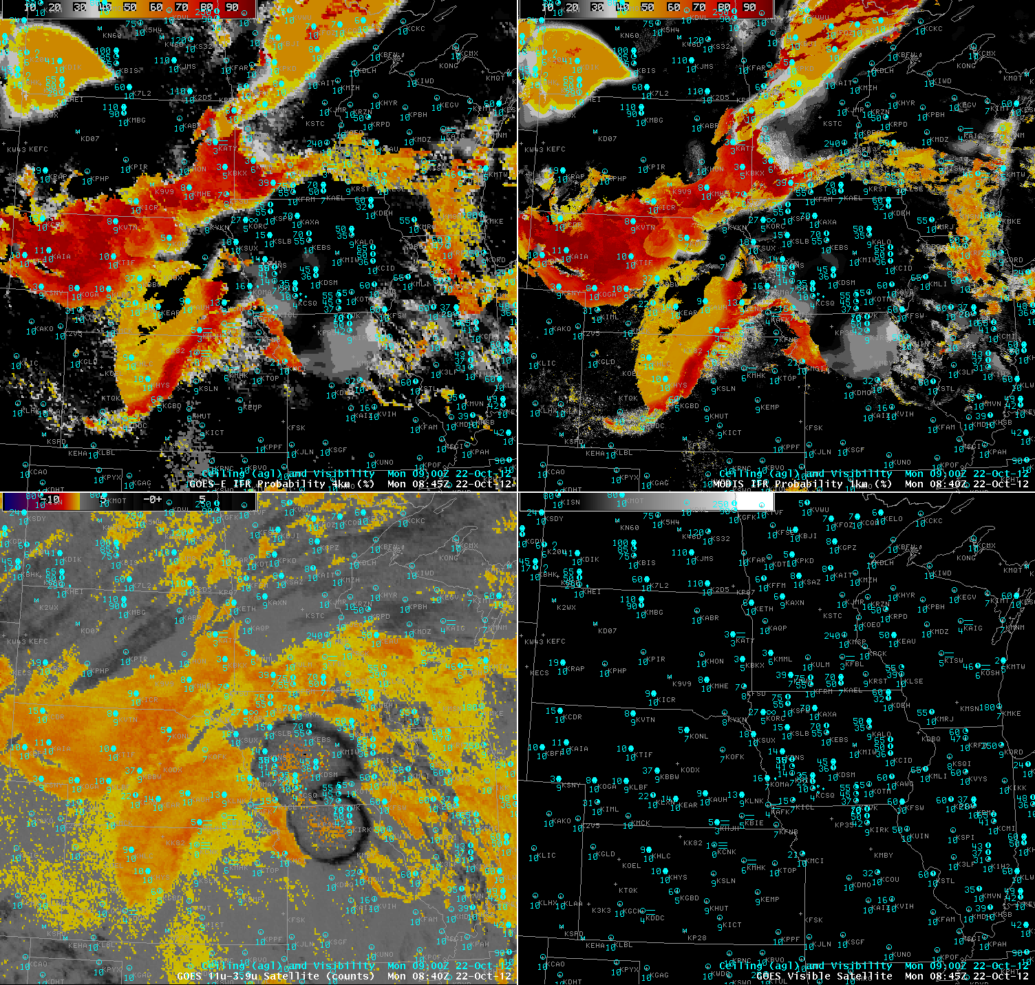
| GOES-R IFR Probabilities (Upper left) and GOES-15 brightness temperature difference (10.7 µm – 3.9 µm) (upper right) from 0900 UTC, Suomi NPP Brightness Temperature Difference (10.8 µm – 3.74 µm) (lower left) |
Ceilings and visibilities decrease further by 0900 UTC, as shown above. Reasons for the difficulty in accurately diagnosing the probabilities over the Salinas Valley can be inferred from the figure above, which includes a (high-resolution) Suomi/NPP Brightness temperature difference plot that has a strong signal all along the Salinas Valley; such a strong signal is not so evident in the GOES brightness temperature difference field that uses data at coarser resolution. It’s important that the satellite signal is strong in this fused product because the valley is not well-resolved in the Rapid Refresh Model. When GOES-R is operational, infrared resolution will be 2 km — in between that of Suomi/NPP (1 km) and GOES (4 km).
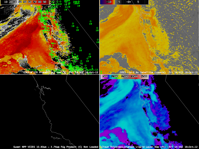 |
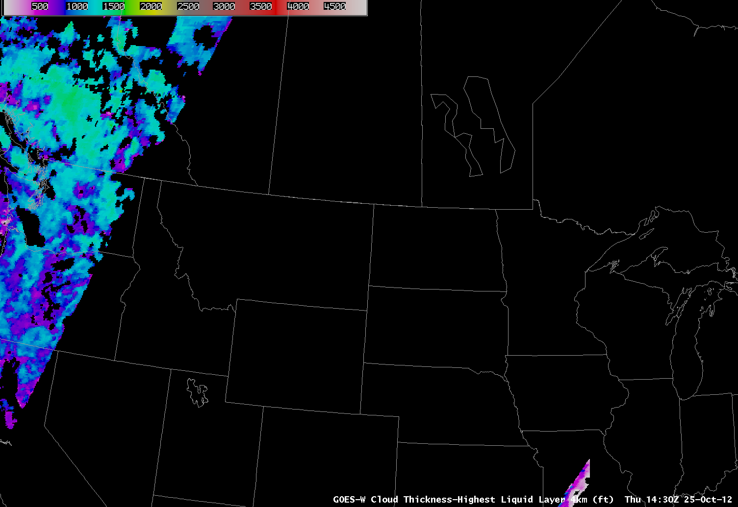
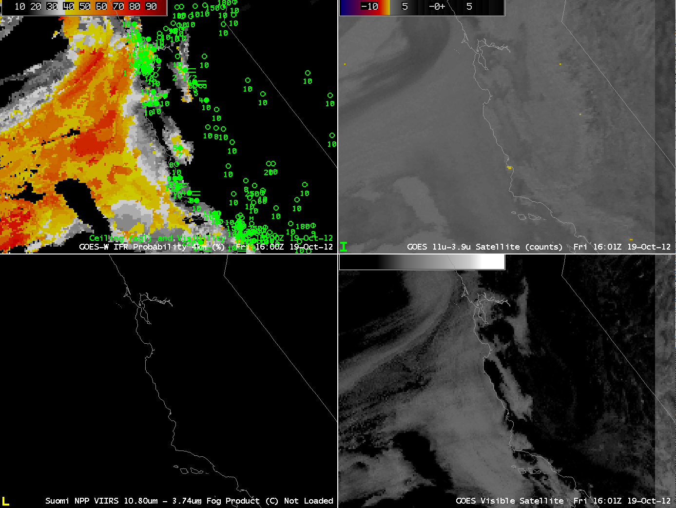
| GOES-R IFR Probabilities (Upper left) and GOES-15 brightness temperature difference (10.7 µm – 3.9 µm) (upper right) from 1400 UTC, GOES-R Cloud Thickness (lower left) |
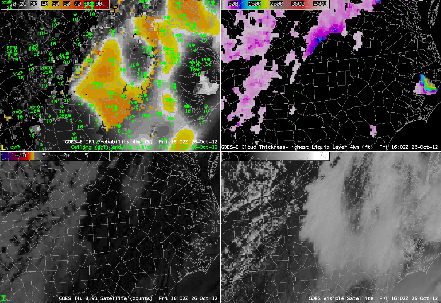
The 1400 UTC image includes cloud thickness as diagnosed by the GOES-R algorithm. Cloud thickness is well correlated with dissipation time for radiation fog — but not necessarily for advection fog. Nevertheless, the regions diagnosed with thickest fog above continue to show fog in the visible imagery below, from 1600 UTC.
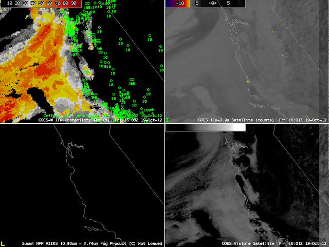 |
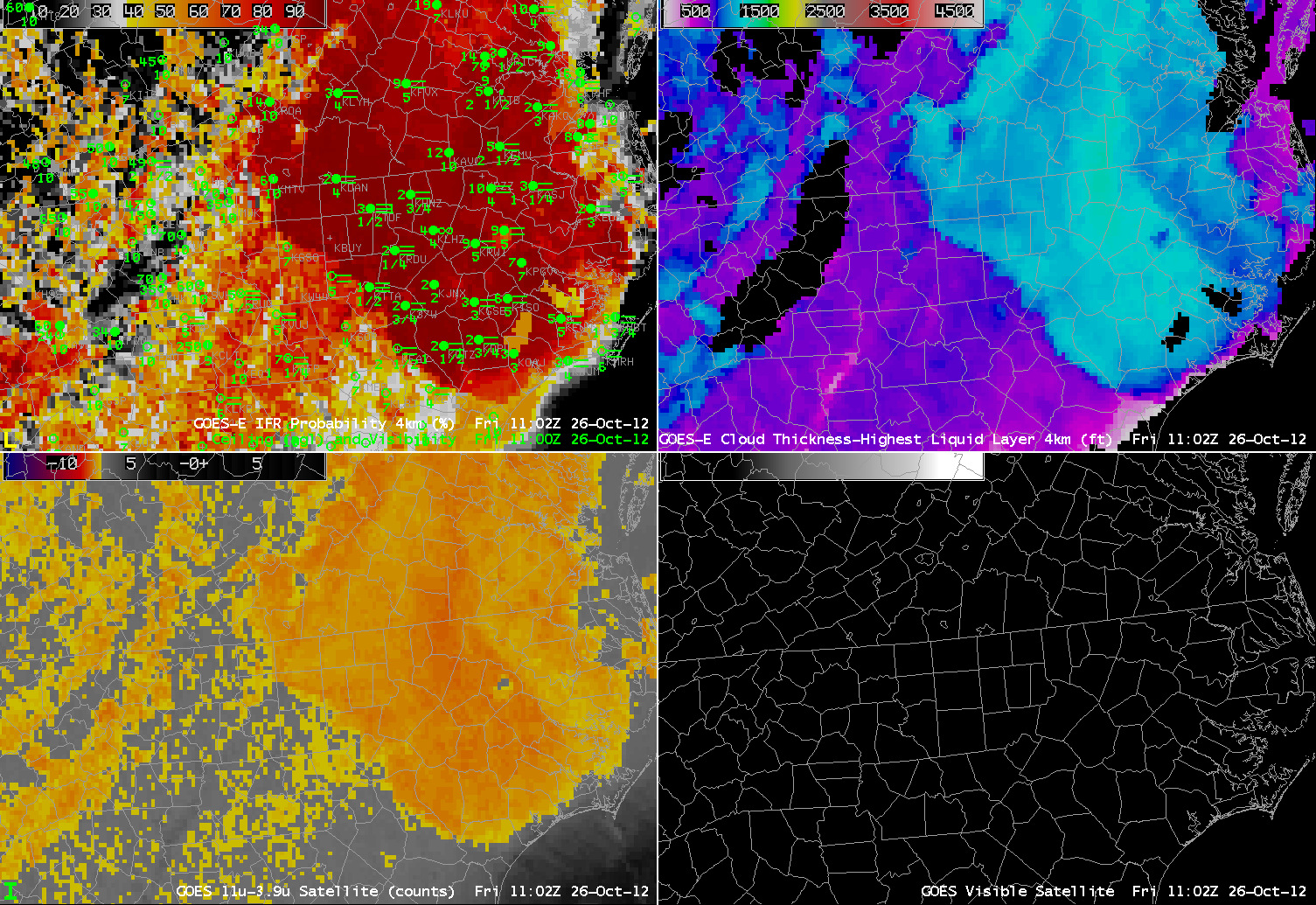
| GOES-R IFR Probabilities (Upper left) and GOES-15 brightness temperature difference (10.7 µm – 3.9 µm) (upper right) from 1400 UTC, GOES-15 Visible Imagery (lower left) |