Category Archives: Dissipation Time

Dense Fog in southern Louisiana

GOES-16 Low IFR Probability fields, 0406 – 1651 UTC, 10 December 2020 , along with surface observations of ceilings and visibility (Click to enlarge)

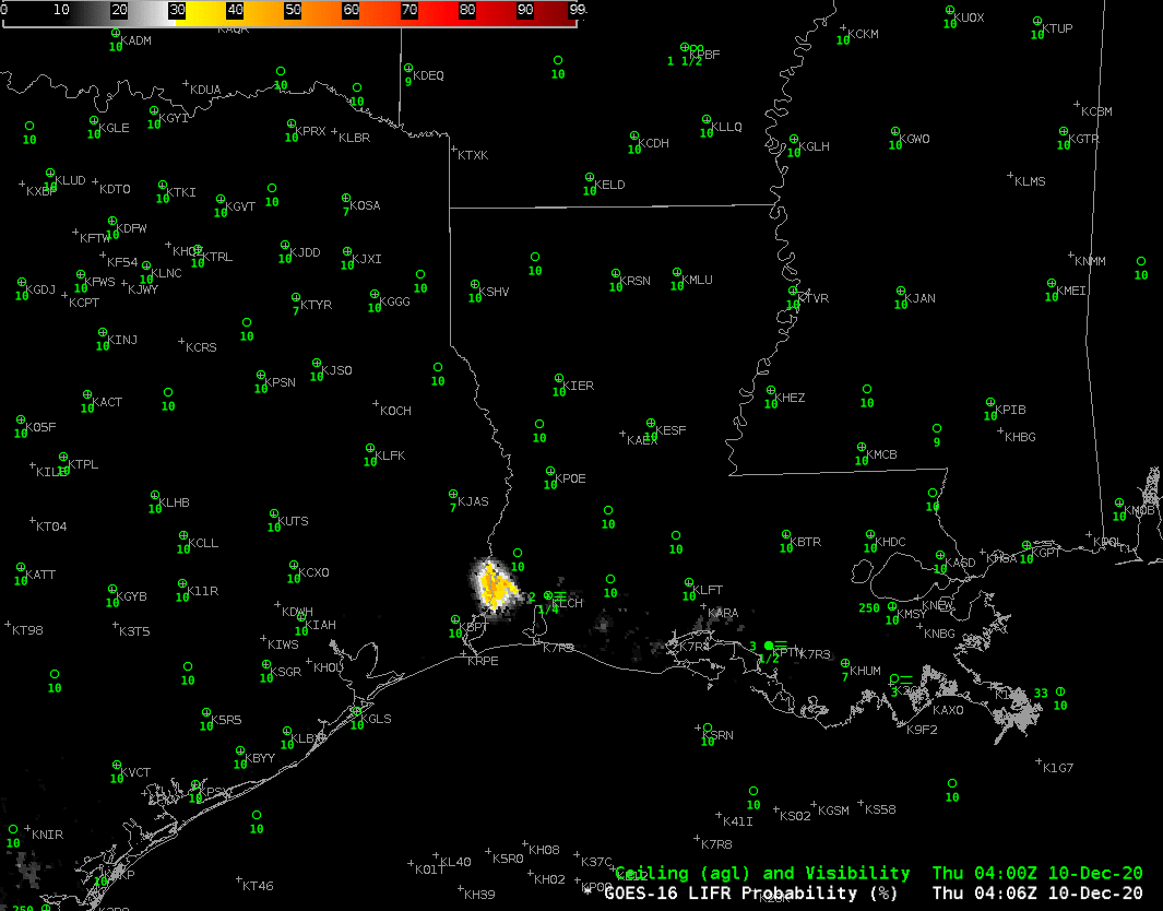
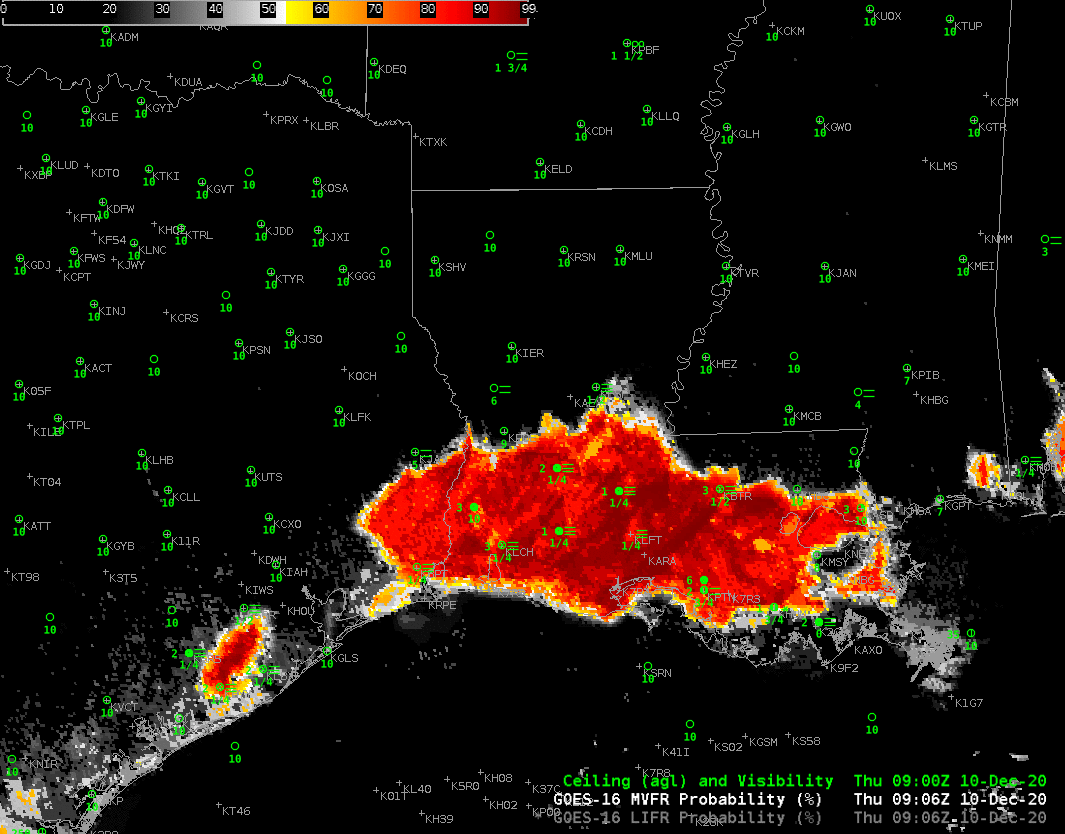
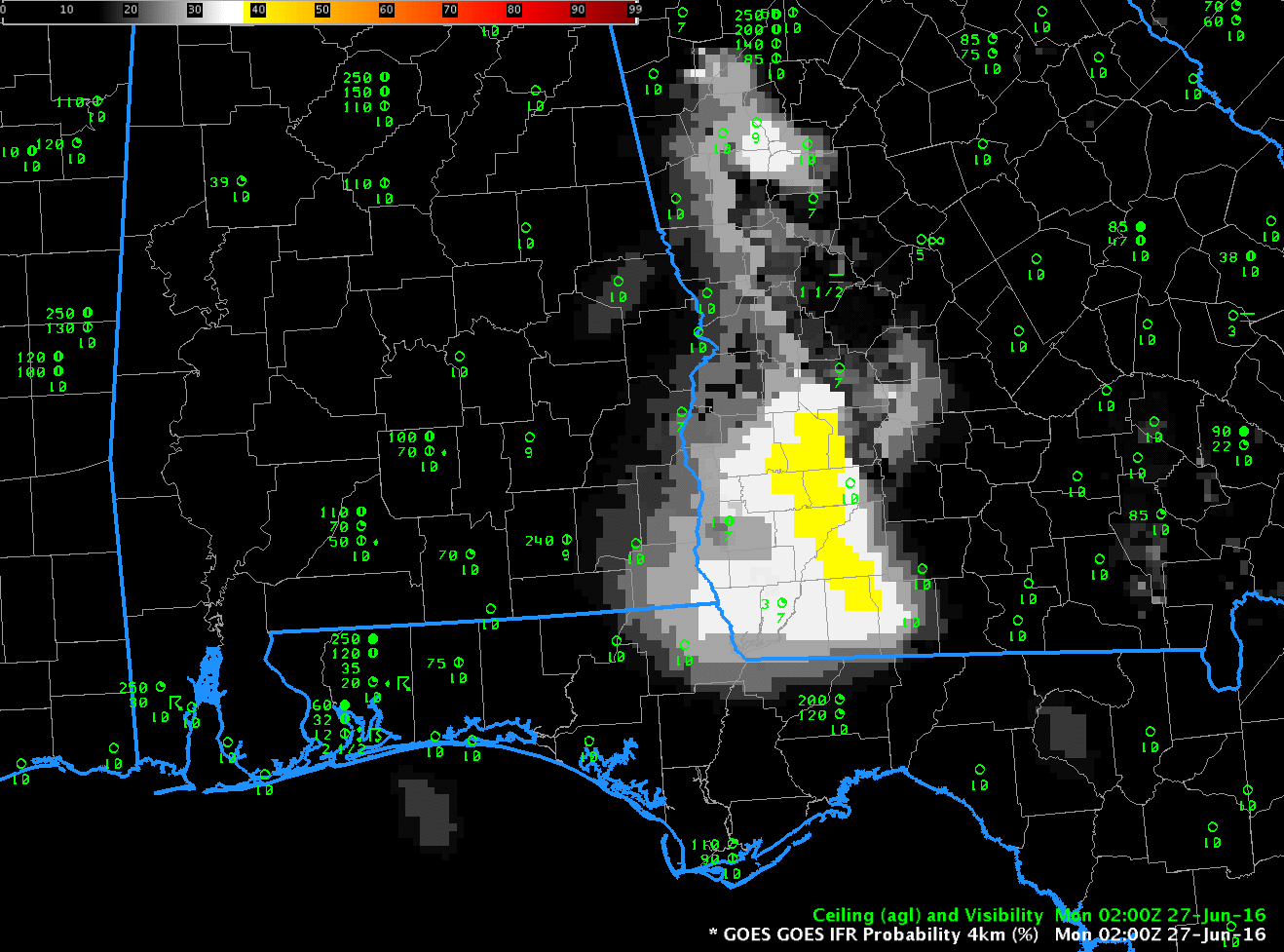
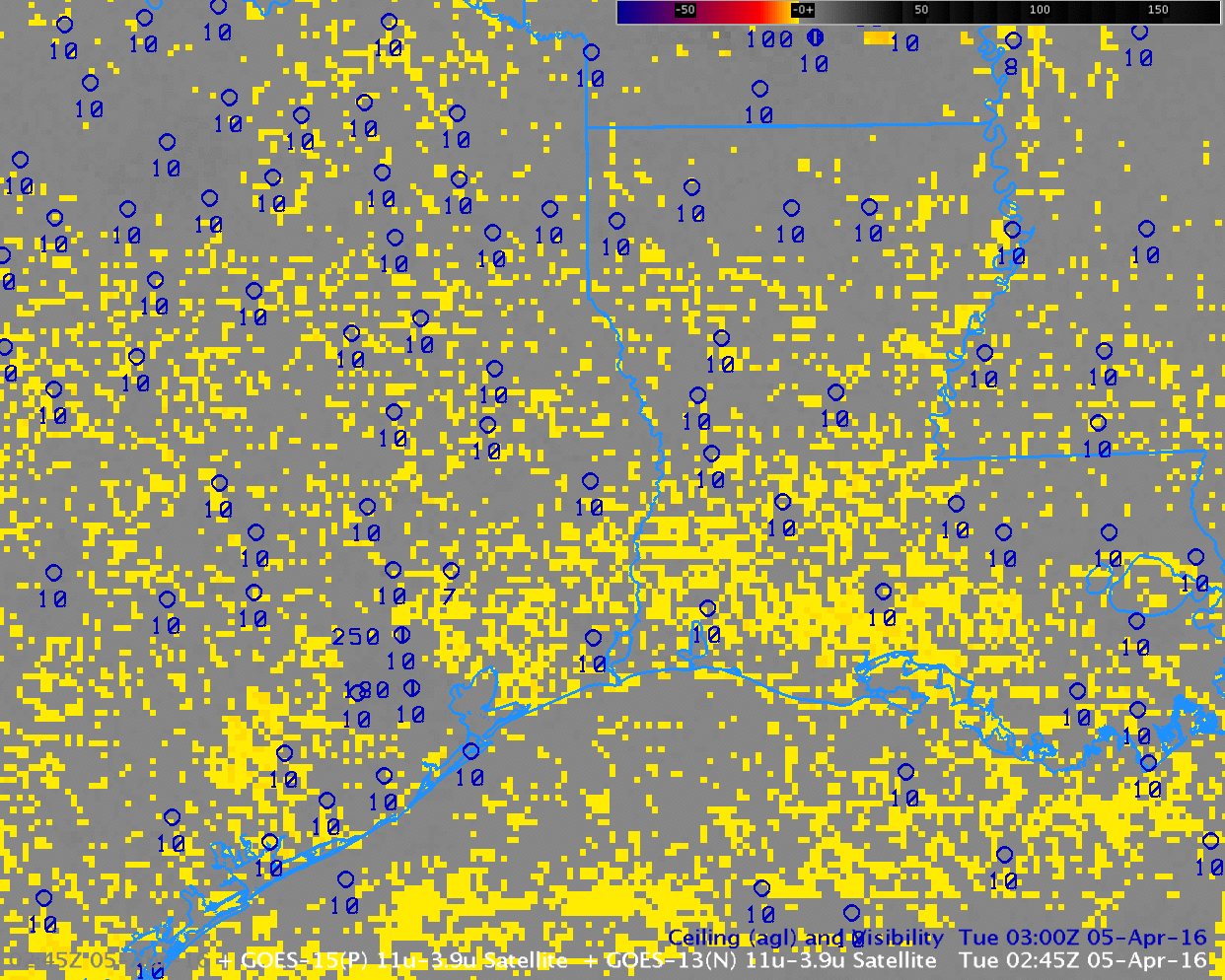
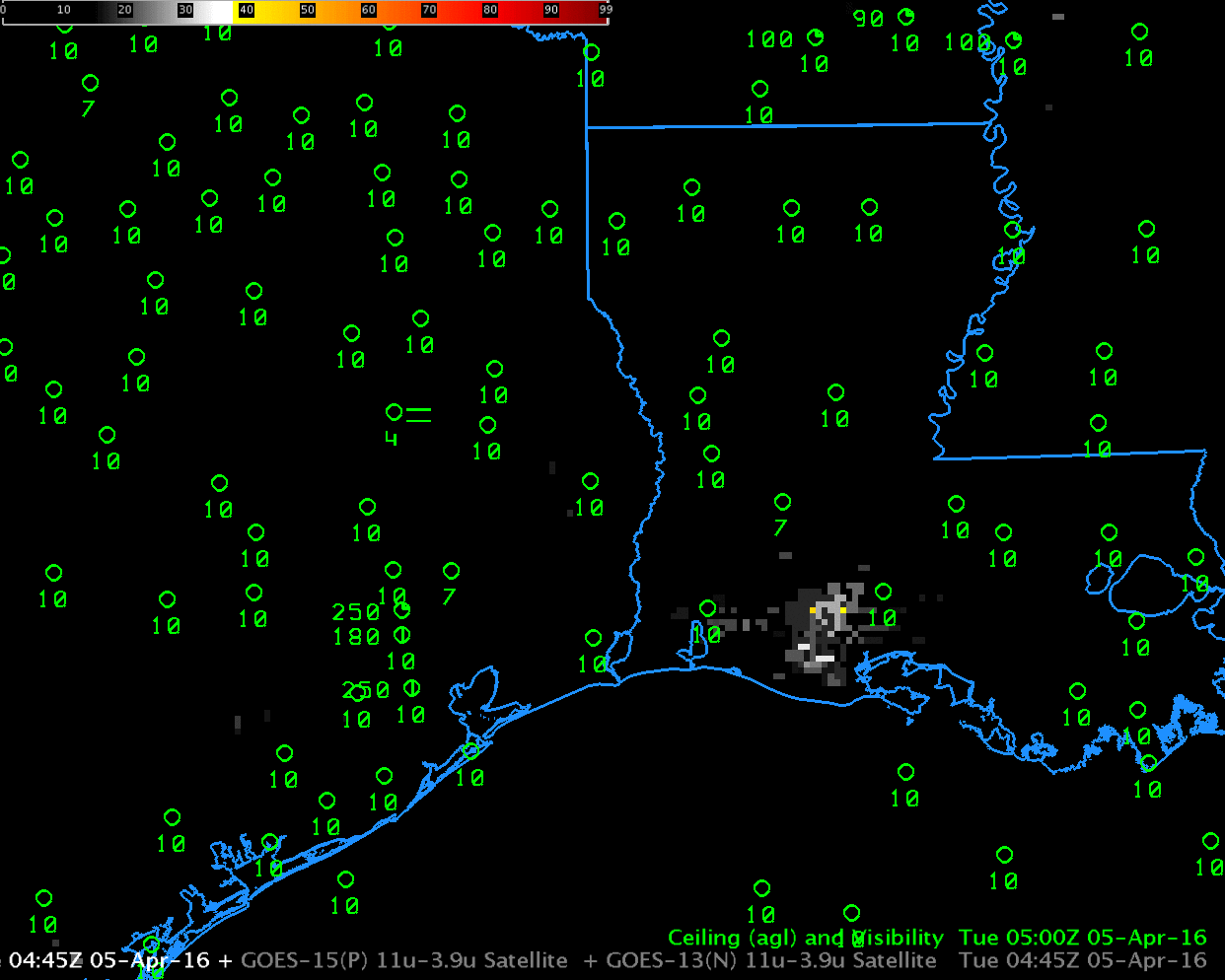
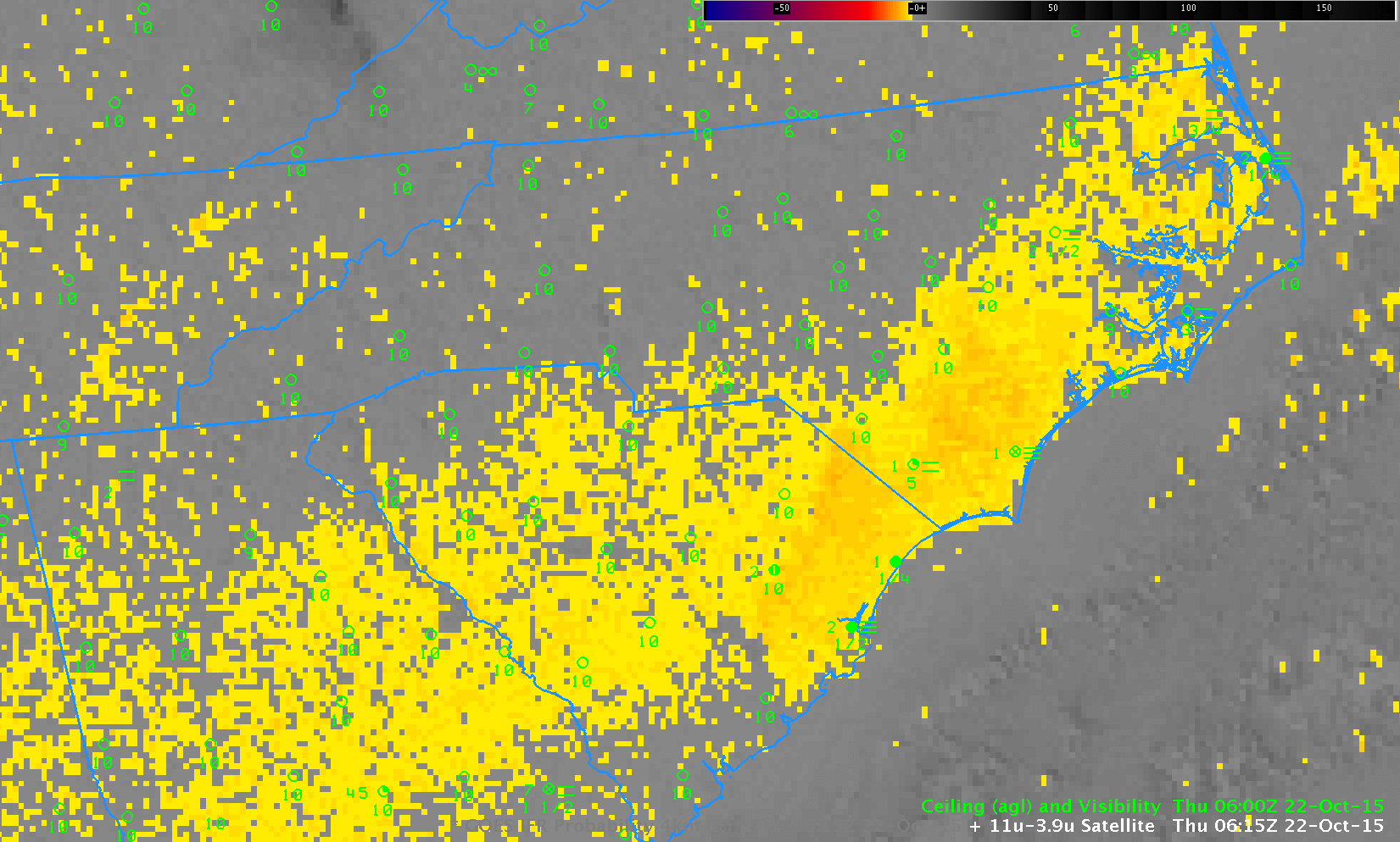
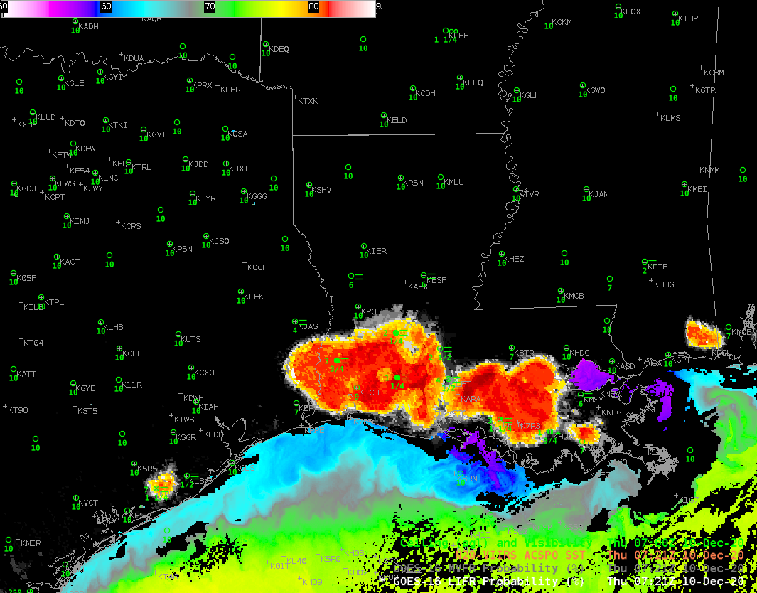
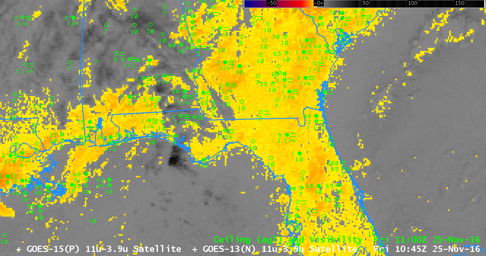
High Pressure (link), cold air, and proximity to warm Sea Surface Temperatures (image here, ACSPO SSTs from the Direct Broadcast Antenna at CIMSS) meant dense fog over southwestern Louisiana. The animation above shows Probabilty of Low IFR Conditions from 0400 UTC through sunrise. Low IFR Probability fields originate near Lake Charles and Franklin before consolidating into one large field over southern Louisiana. Surface observations of ceilings and visibilities also indicate dense fog.

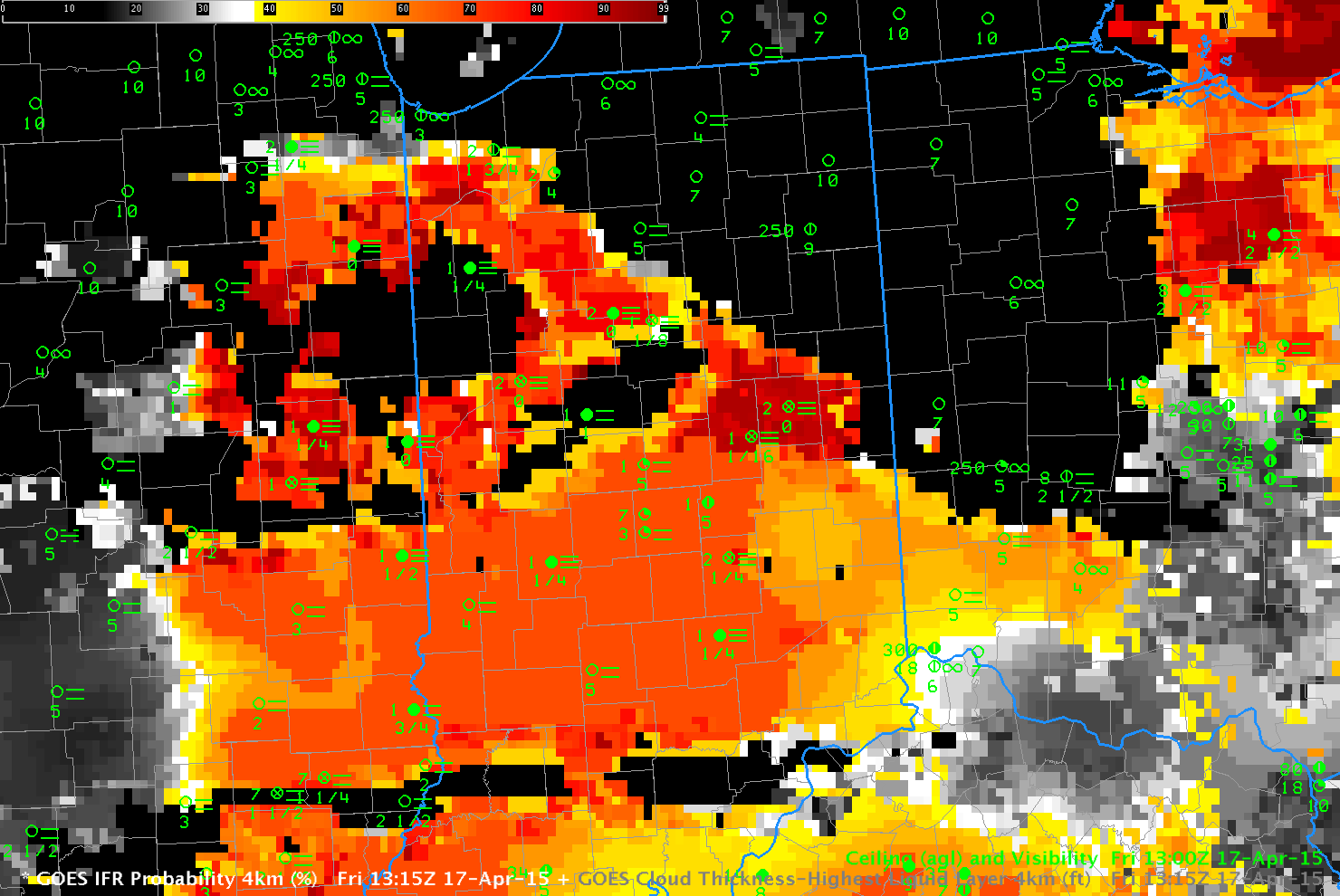
An after-effect of the landfall of Hurricanes is the destruction of webcams that can be used to monitor fog, as noted in the Area Forecast Discussion from WFO Lake Charles, below, from 441 AM CST on 10 December. IFR Probability products in AWIPS combine model predictions of low-level saturation and satellite observations of low cloud to mitigate this loss of information. Regions where low IFR Probability values are high are likely regions that would have dense fog on webcams.

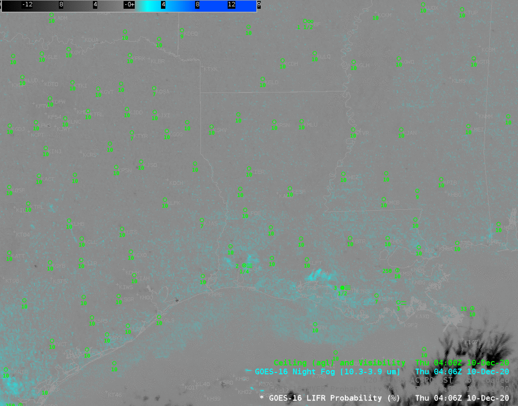
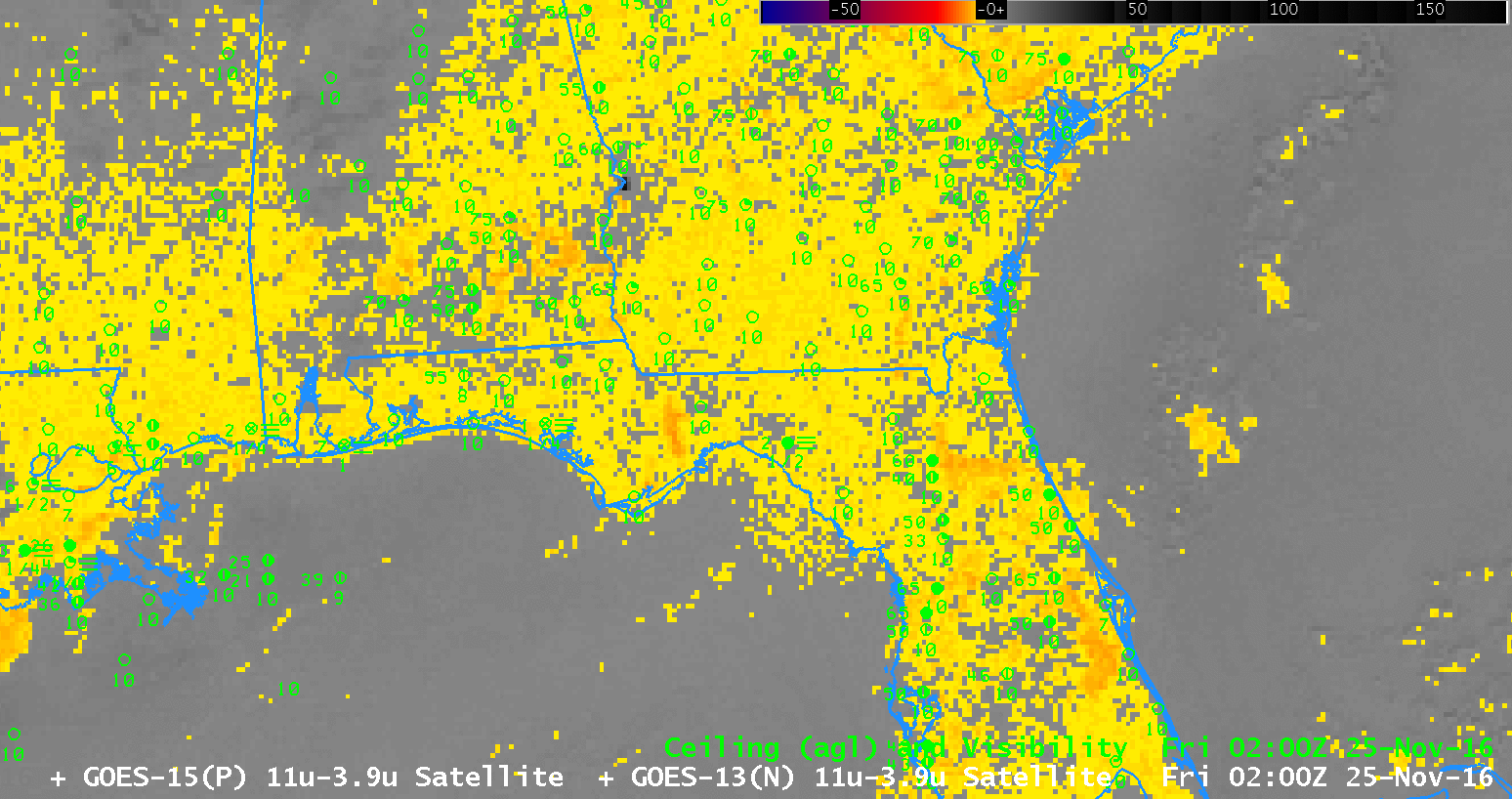
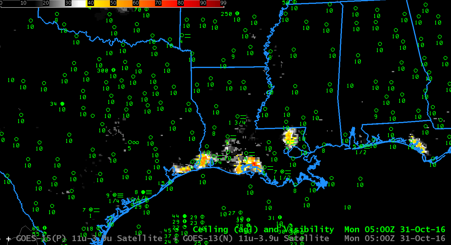
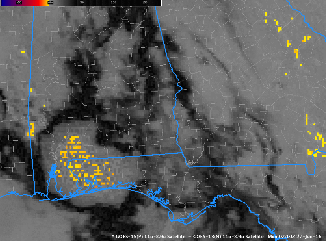
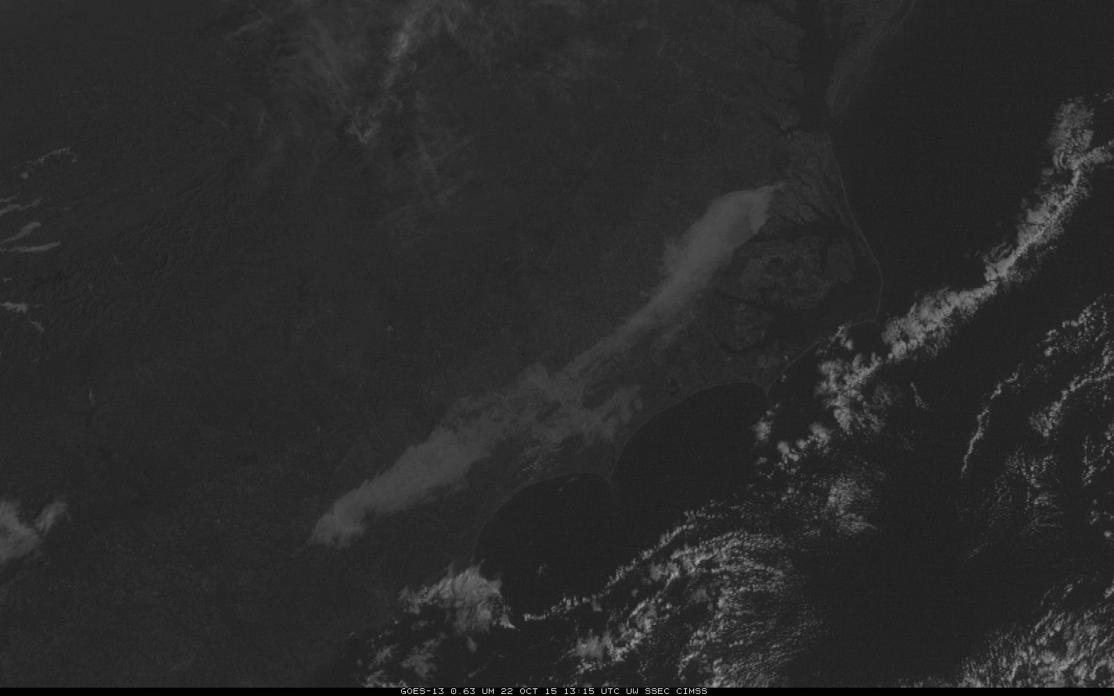
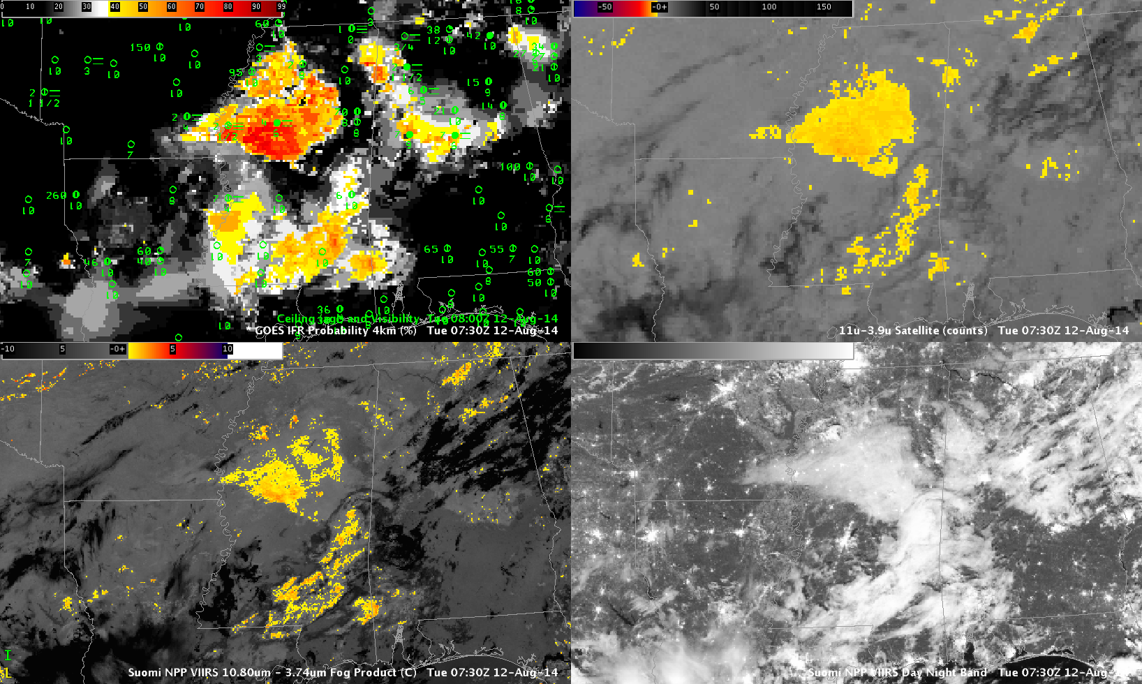
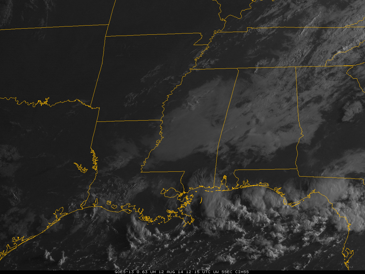
Night Fog Brightness Temperature difference (10.3 µm – 3.9 µm) fields, below, also show the region of stratus clouds. But this satellite-only product does not contain information on how dense the fog is underneath the cloud top (or even if the stratus cloud is also fog). The combination of model data and satellite data by IFR Probability products gives more information than satellite data alone.

GOES-16 Night Fog Brightness Temperature Difference (10.3 µm – 3.9 µm), 0406 – 1651 UTC on 10 December 2020 (Click to enlarge)

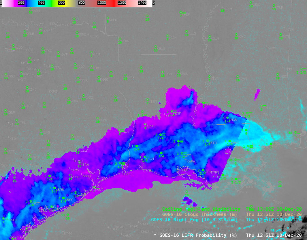
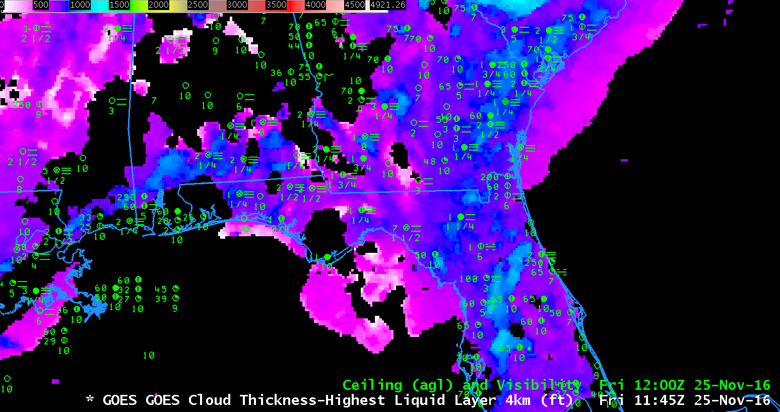
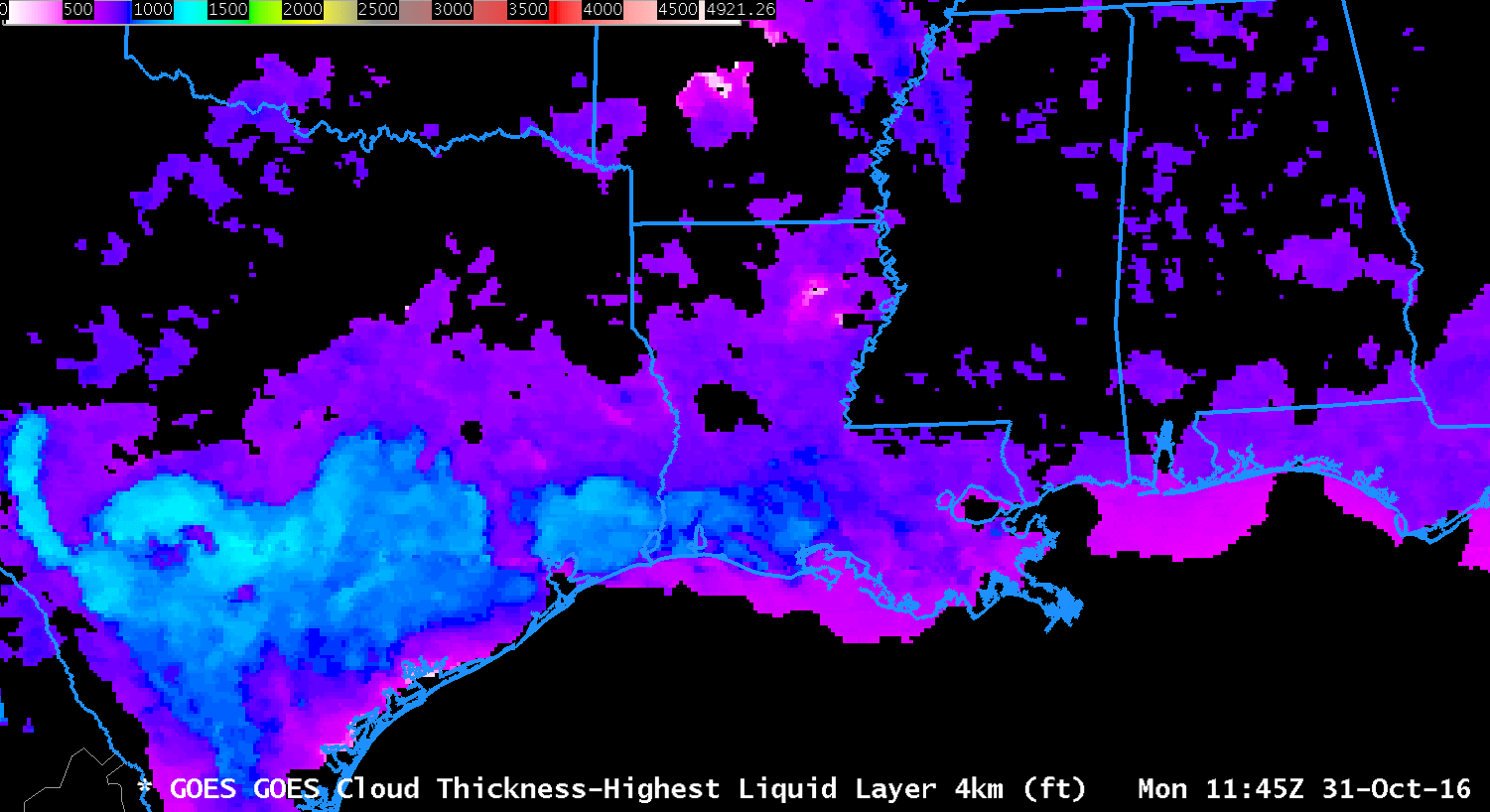
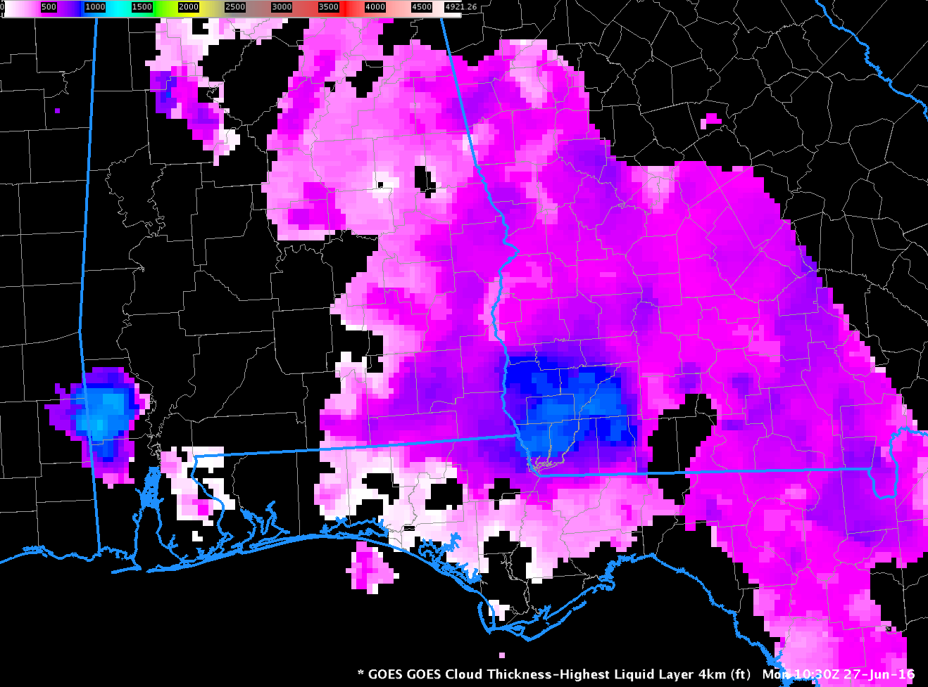
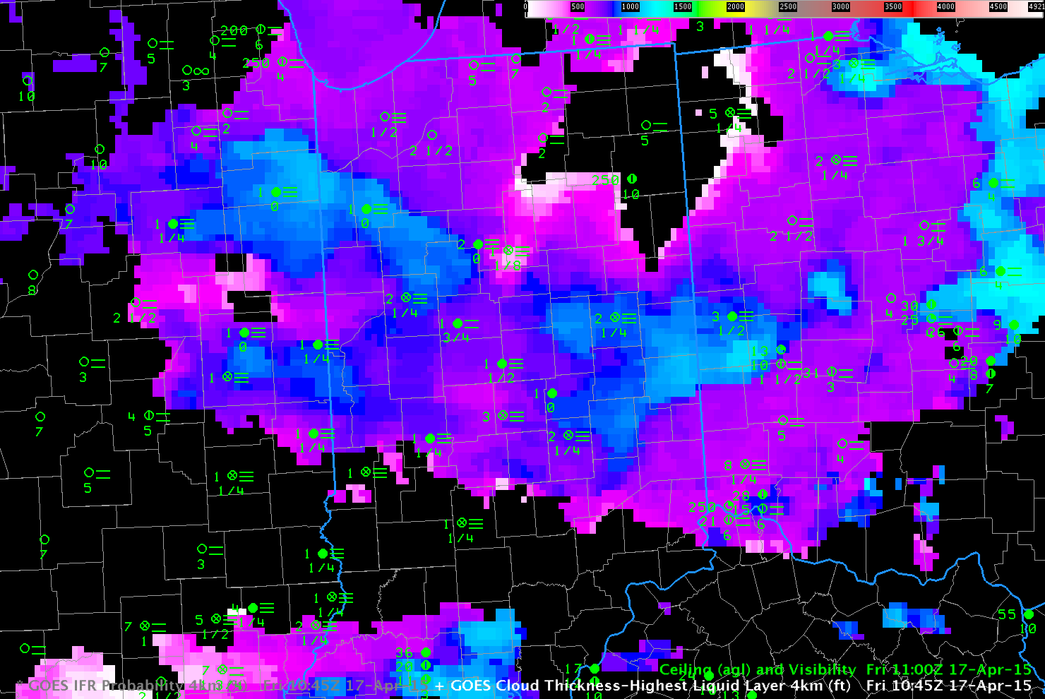
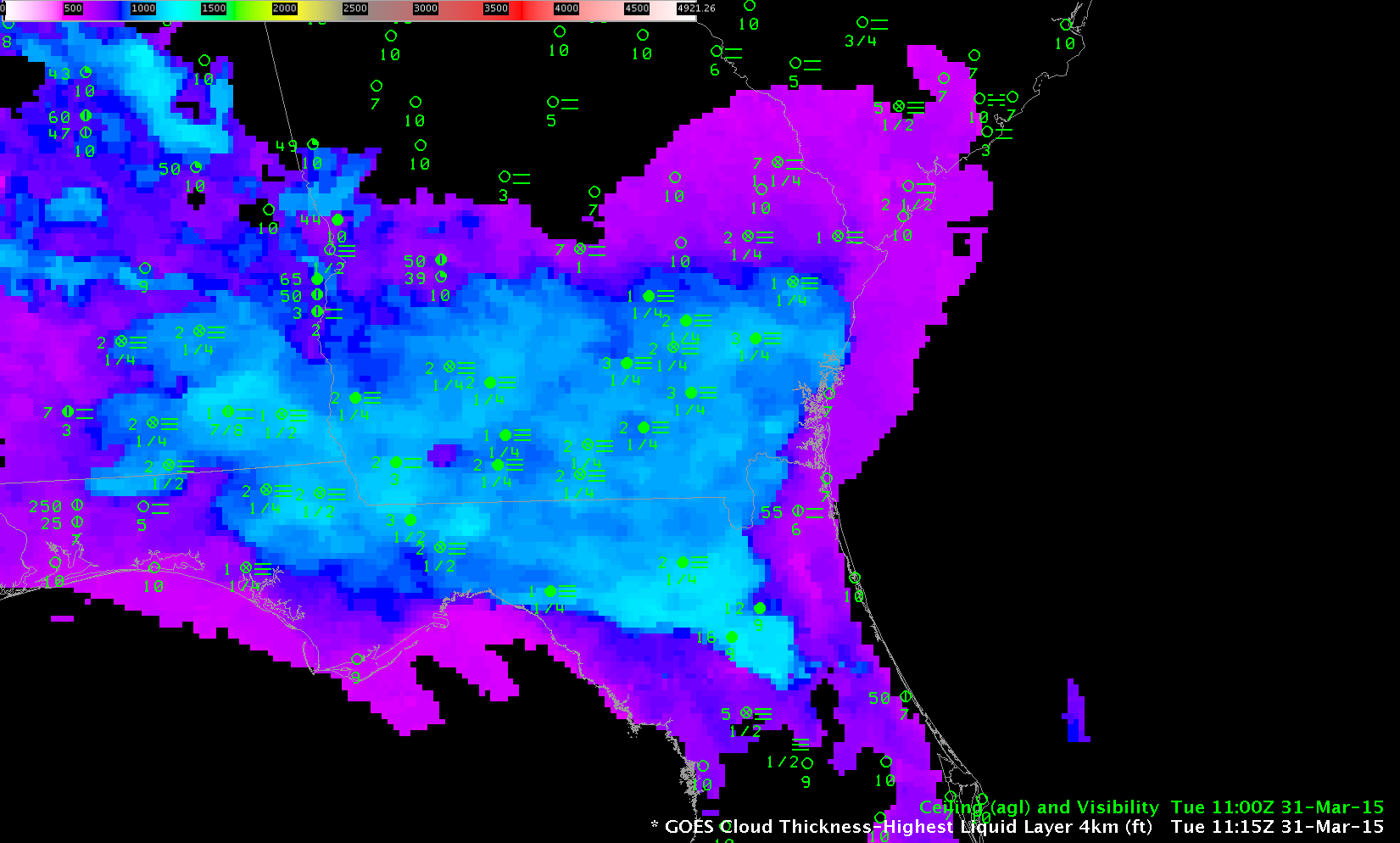
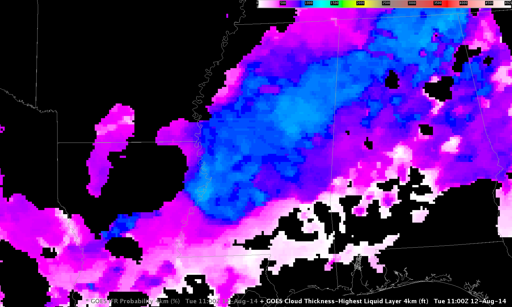
The suite of IFR Probability products includes a GOES-R Cloud Thickness field, shown below overlain on top of a Night Fog Brightness Temperature Difference field. Cloud Thickness is not computed in the 90-120 minutes surrounding sunrise, and the terminator is apparent in the image below, where the Night Fog Brightness Temperature Difference becomes apparent. The thickest cloud (nearly 400 m) is northwest of Lake Ponchartrain. That is where the fog should dissipate last, perhaps.

GOES-R Cloud Thickness field, 1251 UTC, displayed on top of the Night Fog Brightness Temperature Difference field (10.3 µm – 3.9 µm) from the same time (Click to enlarge)

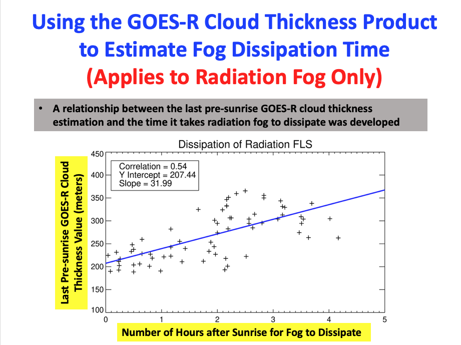
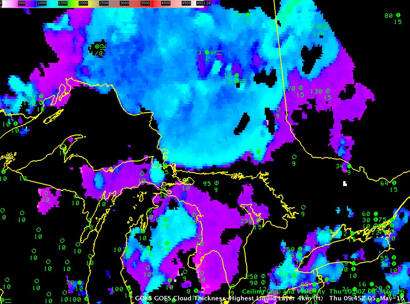
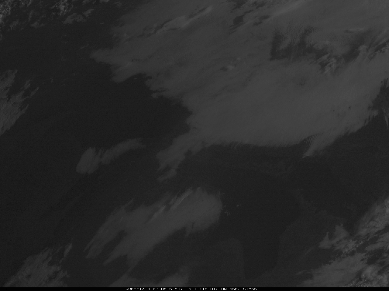
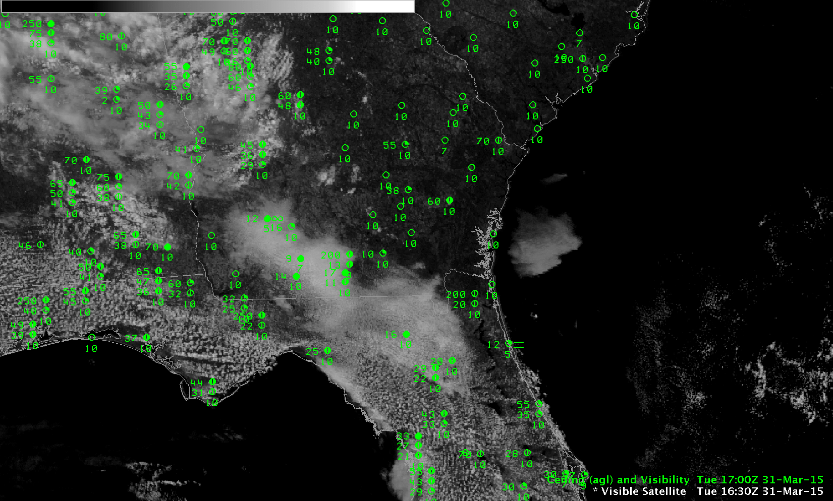
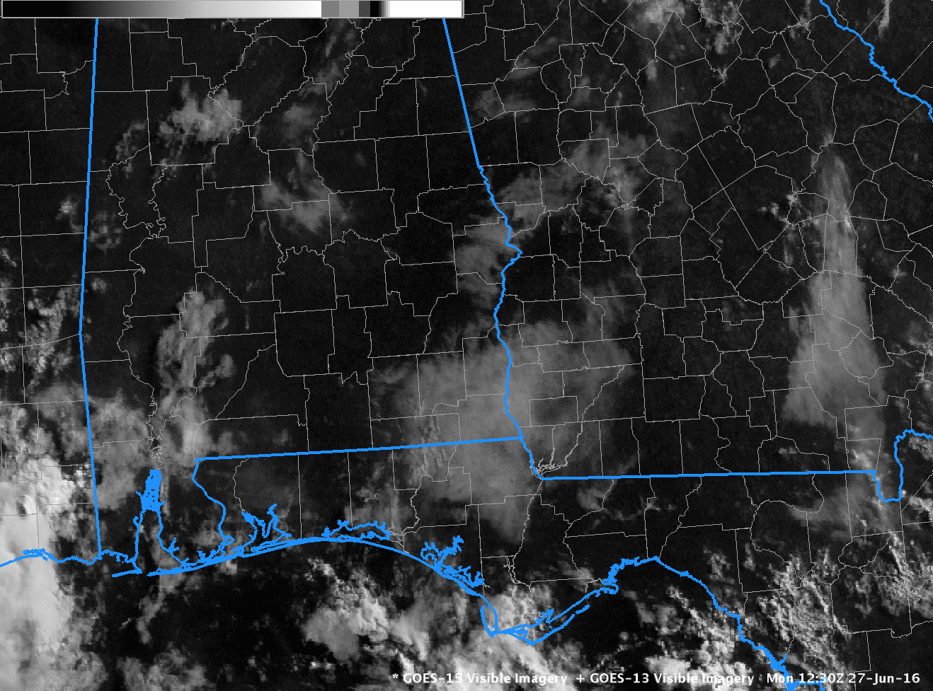
The scatterplot below can be used to estimate when radiation fog might dissipate. It relates the last pre-sunrise observation of GOES-R Cloud Thickness, as shown above, to the number of hours until burn-off. A value of almost 400 m suggests a burnoff nearly four hours after the image above: 1651 UTC. The Thickness field also suggests fog dissipation will be more rapid over southwestern Louisiana than over regions near Lake Ponchartrain. Animations of the Night Fog Brightness Temperature, above, and the visible imagery, below, show that the estimate was a good one on this day.

GOES-16 Band 2 (0.64 µm) visible imagery, 1336 – 1651 UTC on 10 December 2020 (Click to enlarge)

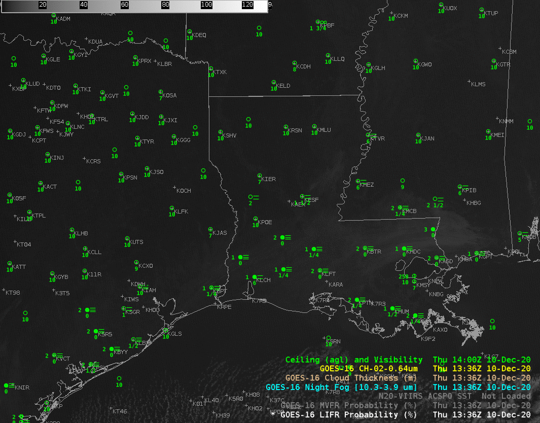
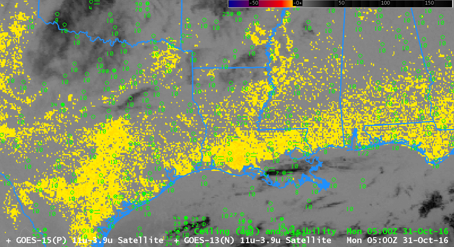
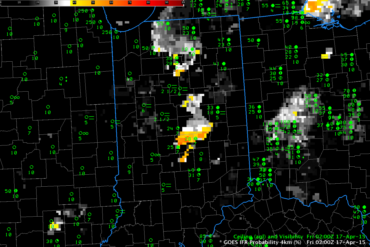
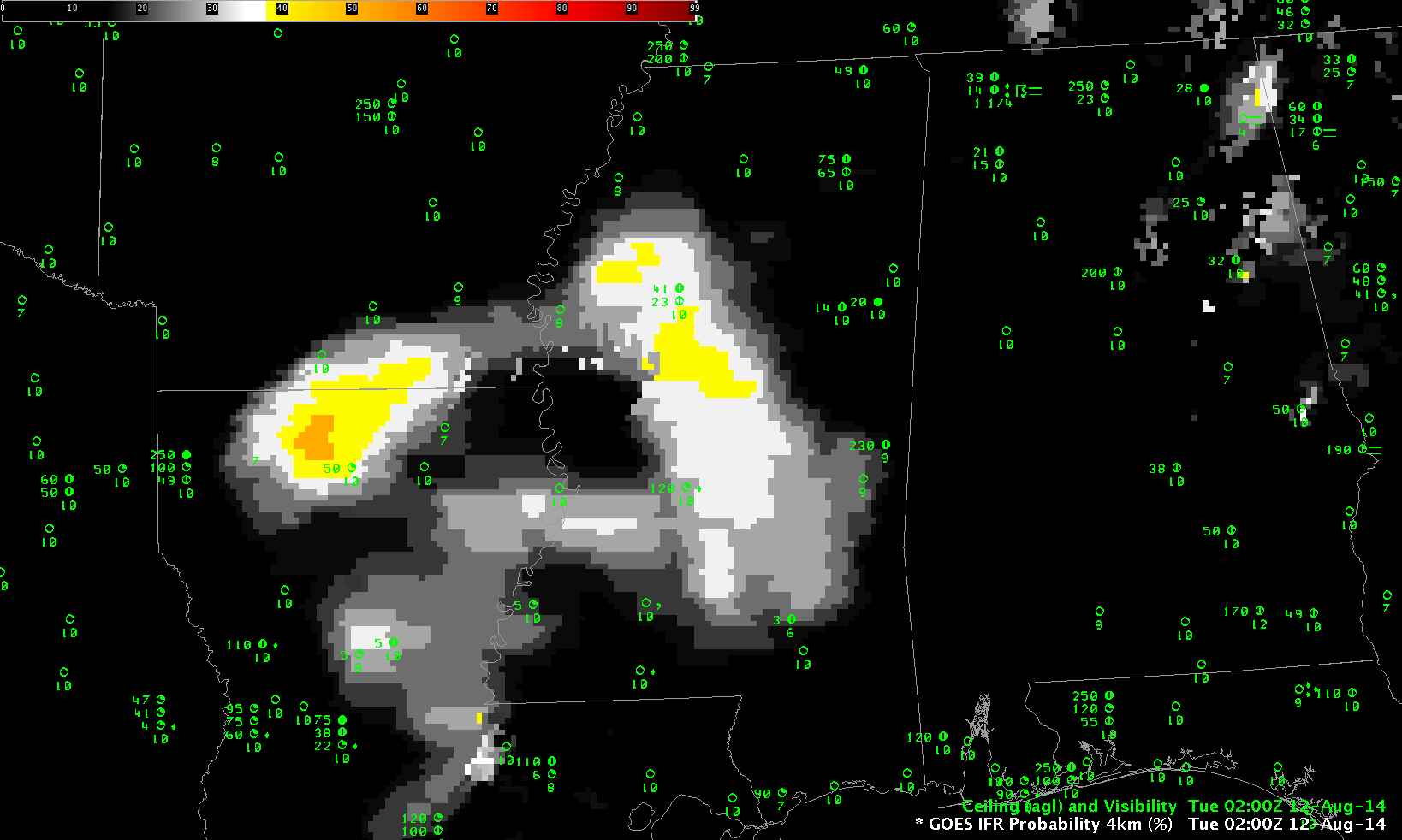
The IFR Probability products include Low IFR Probability, shown above, IFR Probability, and Marginal VFR (MVFR) Probability, in addition to Cloud Thickness. The toggle below, from 0906 UTC, shows that MVFR Probability and Low IFR Probability fields were co-located. As expected, probability of MVFR conditions are greater than probabilities of Low IFR conditions.

GOES-R Low IFR and MVFR Probability, 0906 UTC on 10 December 2020 (Click to enlarge)

Added: Lake Charles WFO also tweeted out this excellent image of a Fog Bow as the fog dissipated!

Dense Fog in Georgia and Florida

ifrprob_25nov2016_0000_1300anim

GOES-R IFR Probability Fields, 0000 – 1300 UTC on 25 November 2016 (Click to enlarge)

Light winds and a long November night allowed radiation fog formation over much of the deep south early on 25 November 2016. (1200 UTC Surface analysis is here). The Aviation Weather Center Website indicated widespread IFR Conditions, below, over the south, with the sigmet suggesting improving visibilities after 1400 UTC.

The animation above shows the evolution of the GOES-R IFR Probability fields from just after sunset to just after sunrise. There is a good spatial match between observed IFR conditions and the developing field. IFR Probability can thus be a good situational awareness tool, identifying regions where IFR Conditions exist, or may be developing presently.

awc_1400utc_25nov2016_ifr

Screenshot of Aviation Weather Center Front Page, 1405 UTC on 25 November (Click to enlarge)

Did the GOES-13 Brightness Temperature Difference Field identify the fields? The animation below, from 0200-1300 UTC, shows a widespread signal that shows no distinguishable correlation with observed IFR conditions.  Note also how the rising sun at the end of the animation changes the difference field as more and more reflected solar radiation with a wavelength of 3.9 µm is present.  In addition, high clouds that move from the west (starting at 0400 UTC over Louisiana) prevent the satellite from viewing low clouds in regions where IFR conditions exist.

btd_25nov2016_0200_1300anim

GOES-13 Brightness Temperature Difference field (3.9 µm – 10.7 µm), 0200-1300 UTC on 25 November 2016 (Click to enlarge)

The high clouds that prevent satellite detection of low clouds, as for example at 1100 UTC over parts of Alabama, cause a noticeable change in the IFR Probability fields, as shown in the toggle below.  Values over the central part of the Florida panhandle are suppressed, and the field itself has a flatter character (compared to the pixelated field over southern Georgia, for example, where high clouds are not present).  Even though high clouds prevent the satellite from providing useful information about low clouds in that region, GOES-R IFR Probability fields can provide useful information because of the fused nature of the product:  Rapid Refresh information adds information about low-level saturation there, so IFR Probability values are large.  In contrast, over southern Florida — near Tampa, for example, Rapid Refresh data does not show saturation, and IFR Probabiities are minimized even through the satellite data has a strong signal — caused by mid-level stratus.  Soundings from Tampa and from Cape Kennedy suggest the saturated layer is around 800 mb.

ifr_btd_25nov2016_1100toggle

GOES-R IFR Probability fields and GOES-13 Brightness Temperature Difference Fields, 1100 UTC on 25 November 2016 (Click to enlarge)

GOES-R Cloud Thickness, below, related 3.9 µm emissivity to cloud thickness via a look-up table that was generated using GOES-West Observations of marine stratus and sodar observations of cloud thickness. The last pre-sunrise thickness field, below, is related to dissipation time via this scatterplot. The largest values in the scene below are around 1000 feet, which value suggests a dissipation time of about 3 hours, or at 1445 UTC.

cloudthickness_25nov2016_1145

GOES-R Cloud Thickness Field, 1145 UTC on 25 November 2016 (Click to enlarge)

IFR Conditions over the Deep South

ifrp_0200_0500_31oct2016anim

GOES-R IFR Probability Fields, 0100-0500 UTC on 31 October 2016 (Click to enlarge)

btd_0200_0500_31oct2016anim

GOES-13 Brightness Temperature Difference Fields (3.9 µm – 10.7 µm), 0100-0500 UTC on 31 October 2016 (Click to enlarge)

Compare the two animation from 0100-0500 above, showing GOES-R IFR Probability fields  (top) and GOES-13 Brightness Temperature Difference fields (bottom) from shortly after sunset on 30 October 2016 until Midnight.  IFR Probability shows very little signal at first, and IFR conditions are rare (Jack Edwards Airport near Gulf Shores AL report IFR conditions).  IFR Probabilities increase slowly in the next 4 hours, especially in regions where IFR conditions develop.  In contrast, the trend in the Brightness Temperature Difference field is a slow decrease in areal coverage with little spatial correlation between a strong signal and IFR reports.  These animations demonstrate a strength of IFR Probabilities:  By combining satellite information with Rapid Refresh predictions of low-level saturation, a better estimate of visibility restrictions can be created.

Subsequent to 0500 UTC, in the animations shown below, IFR Probability fields expanded as IFR conditions developed over western Louisiana and southern/eastern Texas;  a strong signal develops in the brightness temperature difference field in these regions as well.  Note the lack of signal in the GOES-R IFR Probability field over Alabama and Mississippi where Brightness Temperature Difference fields show a consistent signal (and where IFR Conditions are not present).   Brightness Temperature Difference signals over those states may be related to changes in emissivity properties that occur during severe drought, as discussed here.

ifrp_0500-1215_31oct2016anim

GOES-R IFR Probability fields, 0500-1215 UTC on 31 October 2016 (Click to enlarge)

btd_0500-1215_31oct2016anim

GOES-13 Brightness Temperature Difference Fields (3.9 µm – 10.7 µm), 0500-1215 UTC on 31 October 2016

GOES-R Cloud Thickness relates future dissipation of fog to present observations of Cloud Thickness. The last pre-sunrise GOES-R Cloud Thickness field is related to dissipation time in this scatterplot. (GOES-R Cloud Thickness is not computed during twilight times surrounding sunrise and sunset)  The animation below shows the thickest clouds over south-central Texas; fog over Louisiana and coastal Texas is comparatively thin. Dissipation should occur last over interior Texas.

goes-rcloudthickness_1145-1245_31oct2016step

GOES-R Cloud thickness every half hour from 1145-1245 UTC on 31 October 2016 (click to enlarge)

IFR probabilities were noted by the Aviation Weather Center, and Dense Fog Advisories were issued along the Gulf Coast for this case.

Fog/Low Ceilings over Southwest Georgia

GOESR_IFRP_0200_1300_27June2016anim

GOES-R IFR Probability fields on 27 June 2016 at 0200, 0400, and then hourly from 0700 through 1300 UTC (Click to enlarge)

Late-day thunderstorms on 26 June 2016 set the scene for the development of fog overnight over southwestern Georgia. The animation above shows the GOES-R IFR Probability fields.  An enhancement in the fields that is initially driven by Rapid Refresh Model data showing near-saturation at low levels is apparent at 0200 UTC.  As clouds associated with the departing convection dissipate, satellite data could also be used as input into the IFR Probability fields.  The toggle below of GOES-13 Brightness Temperature Difference fields (3.9 µm – 10.7 µm), at 0200 and 0400 UTC, shows the appearance of low-level clouds as mid-level and higher clouds (dark in the enhancement used) dissipate.  By 0400 UTC, when satellite pixels finally start to suggest low clouds, fog had already started to develop.  IFR Probability fields gave an early alert to the possibility of fog development on this day that was not possible from satellite data alone.

GOES_BTD_0200_0400_27June2016toggle

GOES-R Cloud Thickness Fields can give a hint to when radiation fog, as in this event, will dissipate in accordance with this scatterplot. The image below shows the GOES-R Cloud Thickness at 1030 UTC, the last field computed before twilight conditions (indeed, the boundary showing that boundary is readily apparent over eastern Georgia), with values exceeding 900 feet in some places over southwest Georgia.  Based on the scatterplot, that suggests a dissipation time of just over 2 hours (based on the best fit line, but note the scatter in dissipation times associated with cloud thicknesses of 900 feet:  just over an hour to almost 4 hours!) so clear skies would be expected by 1300 UTC.  The animation of visible imagery, here, shows that fog persisted just a bit longer than that, dissipating shortly after 1400 UTC.  GOES-R Cloud Thickness field is an empirical relationship between 3.9 µm emissivity and cloud thickness that is based on SODAR observations off the west coast.  The scatterplot was created based on past observations limited to the southeast part of the US and parts of the Great Plains.

GOESR_CLDT_1030_27June2016

GOES-13 Cloud Thickness, 1030 UTC on 27 June 2016 (Click to enlarge)

Cloud Thickness and Dissipation Time

CloudThickness_0945_05May2016

GOES-R Cloud Thickness, 0945 UTC on 5 May 2016. Note that Cloud Thickness is not computed in the northeast corner where twilight has begun. This is last scene for northern Ontario and Michigan. (Click to enlarge)

GOES-R Cloud Thickness can be used to make a first guess of when fog and low clouds will dissipate. This is done via a look-up table that is derived from this scatterplot. The y-axis on that plot is the last GOES-R Cloud Thickness field produced before sunrise, such as that shown above, and the x-axis is the number of hours after the plot that clearing is expected, GOES-R Cloud Thickness relates 3.9 µm emissivity to dissipation time based on SODAR observations from off the West Coast, and the scatterplot was derived mostly from observations over the southeast US;  the thickness is that of the lowest water-based cloud field and it’s not computed where multiple cloud layers exist — near Geraldton north of Lake Superior, for example, where IFR Conditions are reported — or near sunrise/sunset.  Values are between 1100 and 1200 feet over northern Lower Michigan,  around 1200 feet over eastern upper Michigan, and around 1200 to as much as 1490 feet over northwest Quebec.  The scatterplot suggests a dissipation time of nearly 4 hours, which would be 1345 UTC.

Imagery below shows low clouds persisting just past 1500 UTC.  For this region where the sun angle is not as high as over the southeast US (where most of the observations used for the scatterplot creation were taken), burn-off took a bit longer.  However, note that GOES-R Cloud Thickness did highlight the thickest clouds that took the longest to dissipate;  so, although the scatterplot underestimated the time of dissipation, Cloud Thickness values did identify which regions would clear last.

A final note: GOES-R Cloud Thickness Dissipation times were computed for Radiation Fog Events, such as the one on 5 May 2016. Dissipation of other fogs that create IFR conditions — Advection Fog, Tule Fog — will not be forecast well with this technique.

GOES13VISLoop_1115_1515_5May2016

GOES-13 Visual (0.63 µm) imagery, 1115-1515 UTC on 5 May 2016 (Click to enlarge)

Fog along the Gulf Coast in Louisiana

GOESBTD_0245_1245anim_05Apr2016

GOES-13 Brightness Temperature Difference Fields, every two hours from 0245 to 1245 UTC, 5 April 2016 (Click to enlarge)

Fog developed along the Gulf Coast of western Louisiana overnight. Brightness temperature difference fields have been used in the past to diagnose the development of fog. This capability exists because water-based clouds, such as stratus, have different emissivity properties at 3.9 µm and 10.7 µm. A water-based clouds does not emit 3.9 µm radiation as a blackbody (but it does emit 10.7 µm radiation as a blackbody). Consequently, the computed temperature of the cloud based on the detected 3.9 radiation is cooler than the temperature computed based on the detected 10.7 radiation. The animation above shows the evolution of the brightness temperature difference field, and the field is characterized by a lot of scattershot signal. Some river valley can be inferred in the signal, but the region of fog over southwestern Louisiana does not stand out.

In contrast, the GOES-R IFR Probability field, below, diagnoses an initially isolated region of enhanced IFR probabilities near stations that are reporting reduced ceilings/visibilities.  The enhanced IFR Probabilities develop over southwestern Louisiana and expand outward from there (a second region develops south of Houston TX).  Regions where IFR conditions do not develop have very low IFR Probabilities that persist with time.

GOESIFR_0445_1230anim_05Apr2016

GOES-R IFR Probability Fields, every 2 hours from 0445 to 1230 UTC, 5 April 2016 (Click to enlarge)

GOES-R Cloud Thickness relates 3.9 µm emissivity to cloud thickness based on historical relationships between that value and sodar observations off the west coast of the USA. The value is not computed during twilight conditions on either side of sunrise and sunset, but  the last observation taken before sunrise, shown below, is related to dissipation time according to this scatterplot. Cloud Thickness on the morning of 5 April 2016 was at most 830 feet, suggesting rapid dissipation after sunrise. This is what occurred.

GOESCLDTH_1145_05Apr2016

GOES-R Cloud Thickness, 1145 UTC on 5 April 2016 (Click to enlarge)

Fog in the Carolinas

GOES_IFR_0000_1315_22Oct2015anim

GOES-R IFR Probabilities, hourly from 0000 UTC through 1315 UTC on 22 October 2015 (Click to enlarge)

Dense fog developed over South and North Carolina on the morning of 22 October 2015, just inland from the coast (Click here for screenshot from the National Weather Service homepage from Wilmington NC).  The animation, above, shows the hourly evolution of the GOES-R IFR Probability fields from just after sunset on the 21st through sunrise on the 22nd. Highest probabilities of IFR Conditions overlap the stations where IFR Conditions occur. GOES-R Cloud Thickness also gives information on where the thickest clouds are; the 1115 UTC Cloud Thickness (the final field before twilight conditions change the 3.9 µm emissivity used to diagnose Cloud Thickness) shows the thickest clouds removed from the coast; compare that region to the regions with fog remaining at 1315 UTC in the animation above. There is good overlap. The maximum cloud thickness in the just-before-sunrise image below is a bit over 1000 feet, in northeastern North Carolina; according to this scatterplot that relates pre-sunrise cloud thickness to dissipation time, fog dissipation should occur within 3 hours, that is by 1415 UTC.

GOES_CLDTHK_1115_22Oct2015

GOES-R Cloud Thickness, 1115 UTC on 22 October (Click to enlarge)

IFR Probabilities have better statistics in outlining regions of dense fog. This is because fog that reduces visibility and low stratus that does not reduce visibility can look very similar to a satellite. IFR Probability fields incorporate near-surface information in the guise of Rapid Refresh model predictions of low-level saturation that better refine regions where low stratus extends down to the ground. There are regions where brightness temperature difference has a fog-like signal with high ceilings/good visibility (central South Carolina, for example). These regions have low IFR Probability values because the Rapid Refresh model does not predict low-level saturation. Fusing satellite and model data yields a better product.

GOES_BTD_IFR_0615_22Oct2015toggle

GOES-13 Brightness Temperature Difference (10.7µm – 3.9µm) and IFR Probability fields, 0615 UTC on 22 October 2015 (Click to enlarge)

The visible animation, below, shows that fog dissipated completely shortly after 1430 UTC, in accordance with expectations based on the Cloud Thickness.

GOES13_VIS_22OCT_1315_1445anim

GOES-13 Visible Imagery, 1315 through 1445 UTC on 22 October (Click to enlarge)

Fog over Indiana

IFRPROB_17April2015_02_12

GOES-R IFR Probabilities over Indiana and surrounding states, 0200-1215 UTC on 17 April (Click to enlarge)

For developed over Indiana and surrounding states during the morning of April 17th.  An hourly animation of GOES-R IFR Probabilities, from 0200 through 1215 UTC, computed from GOES-East and Rapid Refresh Data is shown above.  Fog is developing at 0200 UTC, already over portions of western Indiana, and IFR Probabilities increase quickly.  By 0700 UTC, large regions show reduced visibilities and IFR Probabilities exceeding 85%.

High clouds moving in from the west and southwest starting at about 0800 UTC have an impact on the IFR Probability fields as well.  Only Rapid Refresh Data are used to compute IFR Probabilities where mid-level and high clouds prevent satellite detection of low clouds.  As a result, the character of the field changes:  it becomes flatter (less pixelated) and values decrease (because probability is not so certain when satellite data cannot be used to validate Model predictions).

The final image in the animation above, at 1215 UTC, was computed just after sunrise.  Note that IFR Probability values generally increase.  This is especially notable in regions where mid-level and high-level clouds are present (over southern Illinois and southern Indiana).  Probabilities are higher because the satellite can detect clouds are present.  There are also regions at 1215 UTC where IFR Probabilities rapidly drops to zero.  This is likely a difficulty in the Cloud Typing algorithm that occurs with very low sun angle (as discussed here).  Holes at 1215 UTC have filled in by 1300 UTC.

Cloud thickness can give a first estimate of cloud dissipation time. This link shows a scatterplot with a best-fit line that relates dissipation time to Cloud Thickness from a past study. The Cloud Thickness used is the final one computed before twilight conditions, and that is shown below. (Note that cloud thickness is not computed in regions where mid-level and high-level clouds exist) Much of the fog over Indiana is relatively thin — less than 800 feet thick — with a few regions that exceed 1000 feet. Burn-off of this fog should be relatively quick, and most of the Dense Fog Advisories expired at 1400 UTC.

GOESR_CloudThickness_17April_1045UTC

GOES-R Cloud Thickness just before sunrise, 17 April 2015 (Click to enlarge)


URGENT - WEATHER MESSAGE
NATIONAL WEATHER SERVICE NORTHERN INDIANA
600 AM EDT FRI APR 17 2015

INZ020-022-023-032>034-171400-
/O.NEW.KIWX.FG.Y.0005.150417T1000Z-150417T1400Z/
WHITE-CASS IN-MIAMI-GRANT-BLACKFORD-JAY-
INCLUDING THE CITIES OF...MONTICELLO...BROOKSTON...MONON...
LOGANSPORT...ROYAL CENTER...PERU...GRISSOM AFB...MEXICO...
MARION...GAS CITY...UPLAND...HARTFORD CITY...MONTPELIER...
PORTLAND...DUNKIRK
600 AM EDT FRI APR 17 2015

...DENSE FOG ADVISORY IN EFFECT UNTIL 10 AM EDT THIS MORNING...

THE NATIONAL WEATHER SERVICE IN NORTHERN INDIANA HAS ISSUED A
DENSE FOG ADVISORY...WHICH IS IN EFFECT UNTIL 10 AM EDT THIS
MORNING.

* VISIBILITY: A QUARTER MILE OR LESS.

* IMPACTS: VERY HAZARDOUS DRIVING CONDITIONS...WHICH WILL LEAD TO
  TRAVEL DELAYS. PLEASE LEAVE EARLY IF TRAVELING THIS MORNING AND
  ALLOW EXTRA TIME TO REACH YOUR DESTINATION.

PRECAUTIONARY/PREPAREDNESS ACTIONS...

A DENSE FOG ADVISORY MEANS VISIBILITIES WILL FREQUENTLY BE
REDUCED TO LESS THAN ONE QUARTER MILE. IF DRIVING...SLOW DOWN...
USE YOUR HEADLIGHTS...AND LEAVE PLENTY OF DISTANCE AHEAD OF YOU.

Dissipation Time

CloudThickness_1115_31March2015

GOES-R Cloud Thickness over southern Georgia/northern Florida, 1115 UTC on 31 March 2015 (Click to enlarge)

If fog has formed via radiational cooling, the GOES-R Cloud Thickness product that is produced just before sunrise can be used to estimate when clouds will clear. Such an image is shown above for a case of dense fog over southern Georgia on 31 March 2015. The largest Cloud Thicknesses at this time were around 1150 feet over the southern part of this region. Based on this correlation curve, then, dissipation where the fog is thickest should occur 4-1/2 to 5 hours after 1115 UTC. The visible animation below suggests that dissipation was complete by 1715 UTC.

VIS_1630to1730_31March2015

Visible Imagery, 1630-1815 UTC on 31 March 2015 (Click to enlarge)


Fog over Mississippi

FourPanel_0730UTC_12August2014

GOES-R IFR Probabilities computed from GOES-13 at 0730 UTC (Upper Left), GOES-13 Brightness Temperature DIfference (10.7 µm – 3.9 µm) (Upper Right), Suomi NPP VIIRS Brightness Temperature Difference (11.35 µm – 3.74 µm) (Lower Left), Suomi NPP VIIRS Day Night Band (Lower Right), all at 0730 UTC on 12 August 2014

Fog developed overnight in central Mississippi, and the imagery above, at 0730 UTC, is a snapshot during the development. The just-past-full moon provided plenty of illumination, so the stratus and cirrus clouds over the south are distinct. It can be difficult, however, using only the Day Night Band to distinguish between low stratus (north-central Mississippi), mid-level stratus (eastern Mississippi), and high, thick cirrus (Alabama). In addition, the Day Night Band and the brightness temperature difference fields give information at the top of the cloud only. Information about the bottom of the cloud — whether the stratus deck extends to the surface as fog, for example, is difficult to glean from cloud-top properties. This is where the IFR Probability field that incorporates both cloud-top features derived from the brightness temperature difference field and lower-tropospheric information extracted from the Rapid Refresh Model can improve the detection of reduced ceilings and visibilities. Suomi NPP and other polar orbiters can give high spatial resolution imagery. GOES data has excellent temporal resolution to monitor how things evolve with time. The animation below shows how the fog/low stratus developed over the course of the day.

GOES_IFR_Prob_12August2014loop

GOES-R IFR Probabilities and Surface observations of visibility/ceilings, hourly 0200-1100 UTC 12 August 2014

The fields in the animation above change character over the course of the night. Initially, the fields over southwestern Mississippi are very smooth; in this region, multiple cloud layers (a thunderstorm complex was dissipating) prevent any satellite signal from being used as a predictor for IFR Probabilities; only model data are being used. As the night progresses and the mid-level and upper-level clouds dissipate, the character of the field takes on a more pixelated appearance that means satellite data are being used as a predictor. The addition of satellite data to the suite of predictors also means that the probability value increases. By the end of the night, high probabilities have overspread much of central Mississippi, and low ceilings and reduced visibilities are widespread.

GOES-R Cloud Thickness can be used to estimate times of fog dissipation, using the relationship in this scatterplot and the Cloud Thickness in the last pre-sunrise scene, shown below for 12 August 2014. The thickest values are near Vicksburg, MS, where GOES-R Cloud Thickness approaches 1000 feet.  That suggests a clearing time around 1400 UTC, ~3 hours after the valid time of the image below.  The visible animation of the low clouds clearing is below.

CloudThickness_11UTC_12August2014

GOES-R Cloud Thickness, 1100 UTC 12 August 2014

GOES13_KJAN_VIS_12August2014loop