Monthly Archives: June 2014

MODIS-based IFR Probability over California

CA_MODISIFR_0932_30June2014

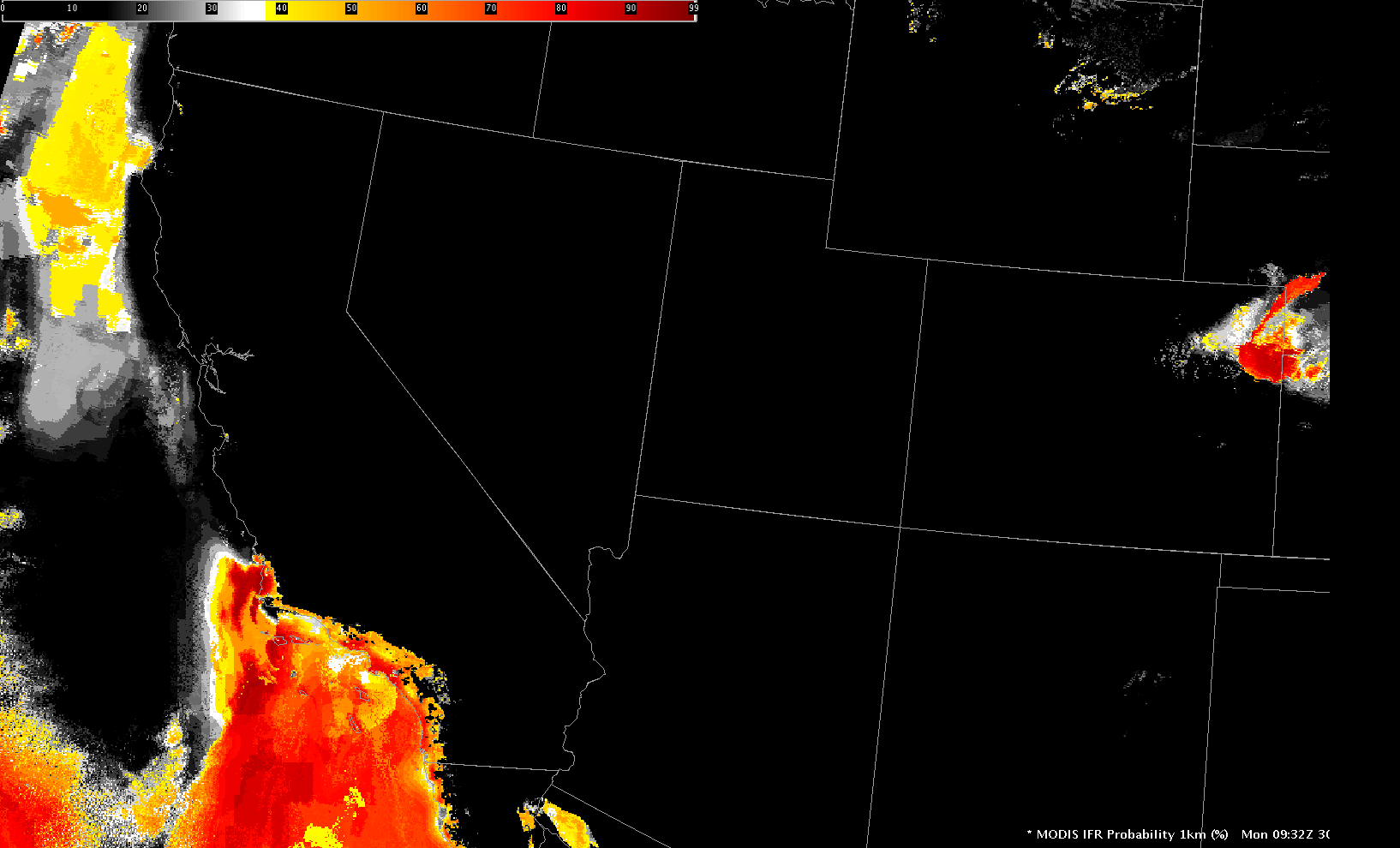
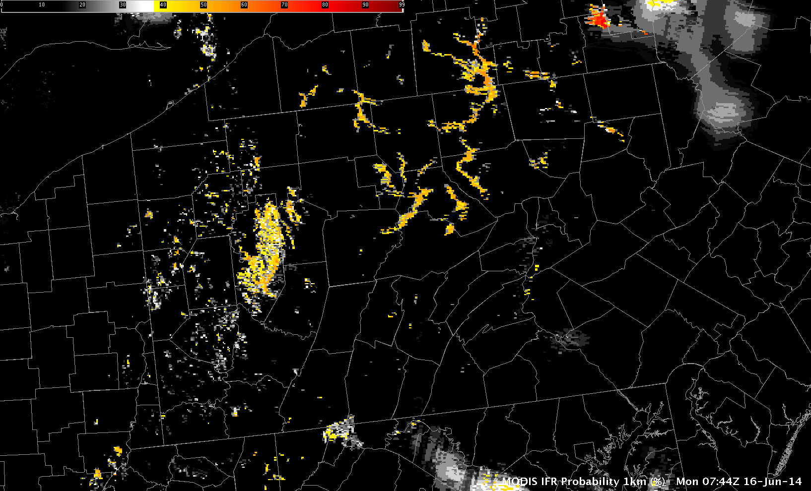
MODIS-based IFR Probabilities over the western US, 0932 UTC on 30 June 2014 (Click to enlarge)

MODIS data, although infrequent, can give a high-resolution estimate of whether of not fog/low clouds are forming in a region. This is particularly useful for cases with highly variable terrain (such as deep river valleys). In the image above, IFR Probabilities are very low over both the Central Valley of California and over the Salinas Valley closer to the coast. Fog/low Stratus are unlikely to be occurring.

CA_SNPPBTD_30June2014_0916_1057

Suomi/NPP Brightness Temperature Difference Fields (11.35µm – 3.74µm) at 0916 and 1057 UTC on 30 June 2014 (Click to enlarge)

The orbital geometry of Suomi/NPP on June 30th was such that it provided two close-up views of these two valleys around/after the time of the MODIS pass shown above. The animation above toggles between those two times. The brightness temperature difference field shows a general increase in return signal strength. But the MODIS IFR Probability field, top, and GOES-West IFR Probability fields (not shown) support the view that any clouds present are not having an impact on ceilings and visibility. A toggle that includes ceilings and visibilities is here.

Note that returns that suggest low clouds over Nevada are more likely due to emissivity differences in different soils, an effect that is more obvious in very dry conditions.

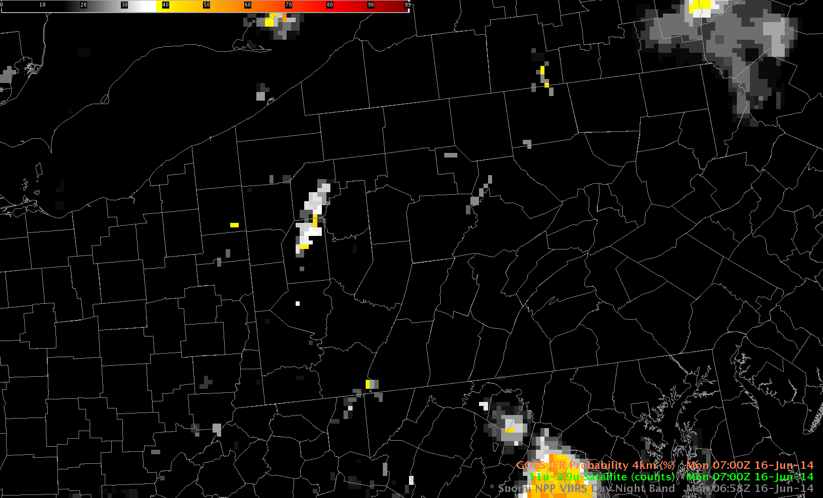
The Suomi/NPP Day/Night band can also provide imagery to help identify the tops of clouds. However, Day/Night Band imagery uses reflected moonlight. There was a new moon on June 27th, and that almost-new moon had set by the time of the images below. Thus, only Earthglow is illuminating any clouds that are present, and that feeble light is mostly overwhelmed by emitted city lights. It is therefore very difficult to identify any changes in cloudcover from the Day/Night band on this date.

CA_30June2014_DNB_0916_1057

Suomi/NPP Day/Night Band imagery at 0916 and 1057 UTC on 30 June 2014 (Click to enlarge)

Fog over Chicago

Chicago_IFRBTD_0915_27June2014

GOES-R IFR Probability and GOES-13 Brightness Temperature Difference, 0915 UTC on 27 June (Click to enlarge)

A cold winter and cool Spring have caused Lake Michigan to be much cooler than normal (Linked-to Figure is on this page). Colder-than-normal lake temperatures and warm summer dewpoints are a recipe for fog, and that fog has persisted over and near Lake Michigan this month. (Click here for a video of fog moving over Chicago on 26 June). The imagery above shows the GOES-R IFR Probability toggling with the GOES-13 Brightness Temperature Difference field (10.7µm – 3.9µm) at 0915 UTC. Abundant high clouds (cirrus from convection over the Plains) makes the brightness temperature difference method of detecting low clouds problematic. Because IFR Probability computation includes surface information, however, a useful signal near Lake Michigan that captures the extent of the fog is produced.

When high clouds prevent satellite predictors from being used, the IFR Probability field is typically fairly smooth. That is the case over most of Lake Michigan. Breaks in the high clouds at 0915 UTC over Chicago allow for satellite predictors to be used. Where that happens, IFR probabilities are larger, and the IFR Probability field is more pixelated.

Click here for a blog entry at the Washington Post on the fog.

Stratus and low Stratus over North Dakota

NoDak_0915_25June2014

GOES-based GOES-R IFR Probabilities (Upper Left), GOES-13 Brightness Temperature Difference (10.7µm – 3.9µm) (Upper Right), GOES-R Cloud Thickness (Lower Left), Suomi/NPP Brightness Temperature Difference (11.35µm – 3.74µm) (Lower Right), all times as indicated (Click to enlarge)

A strength of the GOES-R IFR Probability field is that it highlights regions where IFR conditions are occurring and downplays regions where stratus is elevated off the surface, insignificant from an aviation point of view. In the image above, note how stations in the Missouri River valley of central North Dakota (Bismarck, Mercer County) are under a thick stratus deck that is highlighted in the brightness temperature difference fields, but surface ceilings and visibilities are good. IFR Probabilities there are small because the Rapid Refresh Model data does not suggest low-level saturation. Dickinson and Hettinger, over southwestern North Dakota, in contrast, show restricted visibilities (that worsen before sunrise, see below) in a region of higher IFR Probabilities. IFR Probabilities remain low over central North Dakota where visibilities are not restricted.

NoDak_1015_25June2014

GOES-based GOES-R IFR Probabilities (Upper Left), GOES-13 Brightness Temperature Difference (10.7 – 3.9) (Upper Right), GOES-R Cloud Thickness (Lower Left), Suomi/NPP Brightness Temperature Difference (11.35 – 3.74) (Lower Right), all times as indicated (Click to enlarge)

Fog in the Valleys of Pennsylvania and New York

PA_SNPP_DNB_BTD_0658UTC_16June2014

Suomi/NPP Day/Night Band and Brightness Temperature Difference (11.35 – 3.74) at 0658 UTC on 16 June 2014 (Click to enlarge)

Suomi/NPP Day/Night band “Visible Imagery at Night” from last night at 3 AM EDT over Pennsylvania and surrounding states shows cloud formation in the river valleys of Pennsylvania and New York. The brightness temperature difference also shows these cloud formations, but note over eastern New York how high cirrus prevents the detection of low clouds in river valleys using the brightness temperature difference field, but the cirrus is thin enough that the Day/Night band does show the low clouds. The brightness temperature difference field can show where clouds are present in regions where city lights in the day/night band might appear similar to clouds on a night when lunar illumination is strong (as was the case on 16 June 2014) — for example, along US Highway 220 from Lock Haven to Jersey Shore and Williamsport in southern Clinton and Lycoming Counties.

Of course, the Suomi/NPP satellite is seeing the top of the cloud, so it can be difficult to infer ceiling and visibility obstructions from these data. The GOES-based IFR Probability field from about the same time, below, shows hints of visibility restrictions, but the coarser resolution of GOES-13 (compared to Suomi/NPP) limits the ability of GOES to herald the development of fog. In addition, the 13-km resolution of the Rapid Refresh model data that are also used in the GOES-R IFR Probability fields is insufficient to resolve the small river valleys (such as Pine Creek that shows up very well in the S/NPP imagery in western Lycoming County). Portions of the Susquehanna River basins do show marginally enhanced probabilities, certainly something that would alert a forecaster to the possibilities of fog.

PA_IFRProbGOES_0700UTC_16June2014

GOES-based IFR Probabilities, 0700 UTC on 16 June 2014 (Click to enlarge)

MODIS data can also be used to produce IFR Probabilities at infrequent intervals, but a timely overpass at 0744 UTC shows high probabilities in most of the river valleys of central Pennsylvania and upstate New York, with the highest probabilities near Elmira, NY.

MODIS_IFR_0744UTC_16June2014

MODIS-based IFR Probabilities, 0744 UTC on 16 June 2014 (Click to enlarge)

The GOES-R IFR Probabilities at 1000 UTC, below, show evidence that the fog/low stratus have become widespread enough in river valleys to be detected even by GOES. Elmira, NY, is reporting IFR conditions, and such conditions are also likely elsewhere in the valleys (although no observations are available to confirm that).

PA_IFRPROB_1000UTC_16June2014

GOES-based IFR Probabilities, 1000 UTC on 16 June 2014 (Click to enlarge)

Use timely polar-orbiting satellite data — with high resolution — to confirm suspicions of developing fog in river valleys. Then monitor the situation with the good temporal resolution of GOES. During the GOES-R era, geostationary satellite spatial resolution will be increased and fog detection from GOES-R should occur with better lead time.

Colorbars

IFR_LIFR_MVFR

GOES-R IFR Probabilities (Upper Left), GOES-R Low IFR Probabilities (Upper Right), GOES-R MVFR Probabilities (Lower Left) and GOES-R Cloud Thickness (Lower Right), time as indicated (Click to enlarge)

The default colorbars for GOES-R IFR (Instrument Flight Rules) Probabilities, Low IFR Probabilities and MVFR (Mostly Visible Flight Rules) Probabilities change colors at different break points, as shown above (by where the arrows are, for example). IFR Probabilities switch from white to orange/yellow at around 40%, vs. 30% for LIFR and 55% for MVFR. A statistical analysis of the surface observations was used in the development of the colorbars. Highest skill at detecting the category was assigned the reddest colors. One could therefore infer from this that there is in general less skill in detecting MVFR conditions than LIFR conditions. For a given event, however, as shown above, MVFR probabilities will in general be larger than IFR or LIFR probabilities.

Let the color of the colorbar guide the interpretation. Black and white values mean the category (IFR conditions, for example) is unlikely, yellow means it’s possible, and red means it is highly likely. MVFR probabilities have higher thresholds than LIFR probabilities because of skill differences in predicting the different visibilities associated with the sky conditions.