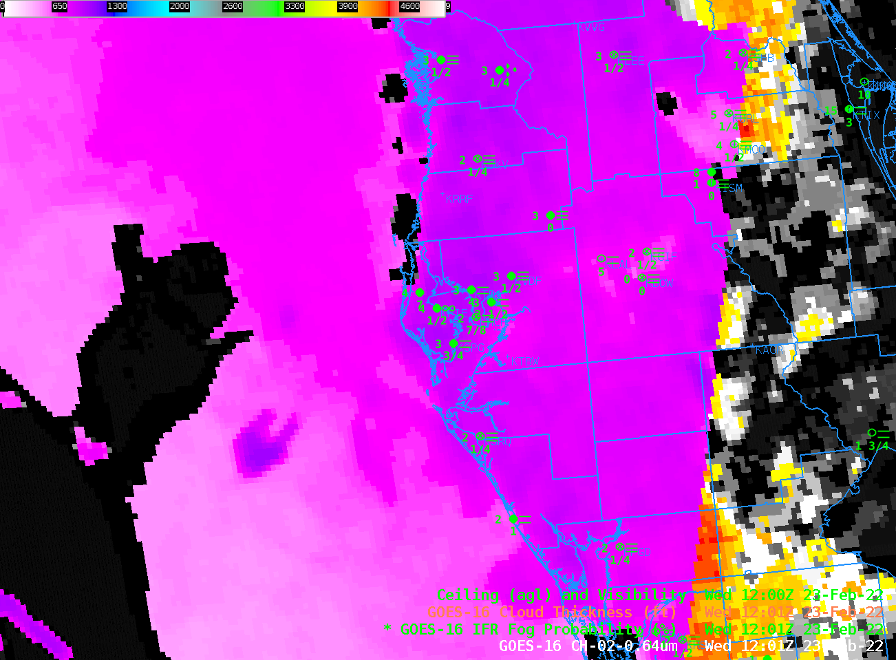
The animation below shows IFR Probability fields layered on top of visible imagery. Early morning fog that reduced visibilities and ceilings to sub-IFR conditions are indicated over much of the middle of the Florida peninsula. (Note that the IFR Probabilty color enhancement was altered so that it was transparent for values < 20%, allowing the visible imagery beneath to appear).
GOES-16 IFR Probability Fields and Visible Band 2 (0.64 µm) imagery, 1151 – 1506 UTC (Click to enlarge)
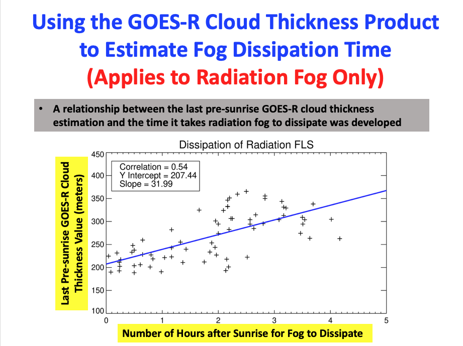
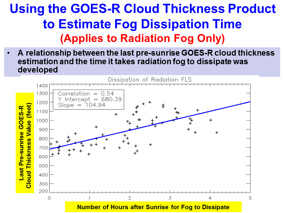
GOES-16 Cloud Thickness fields, below, depict a shallow fog: thickness values in general are under 1000 feet. This scatterplot relates the last pre-sunrise Cloud Thickness — in meters! — to burn-off time; a value of 1000 feet will burn off very quickly as observed above.
Cloud Thickness at 1201 UTC on 23 February 2022 (Click to enlarge)
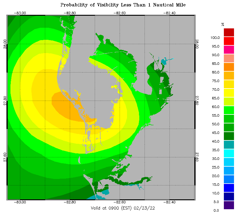
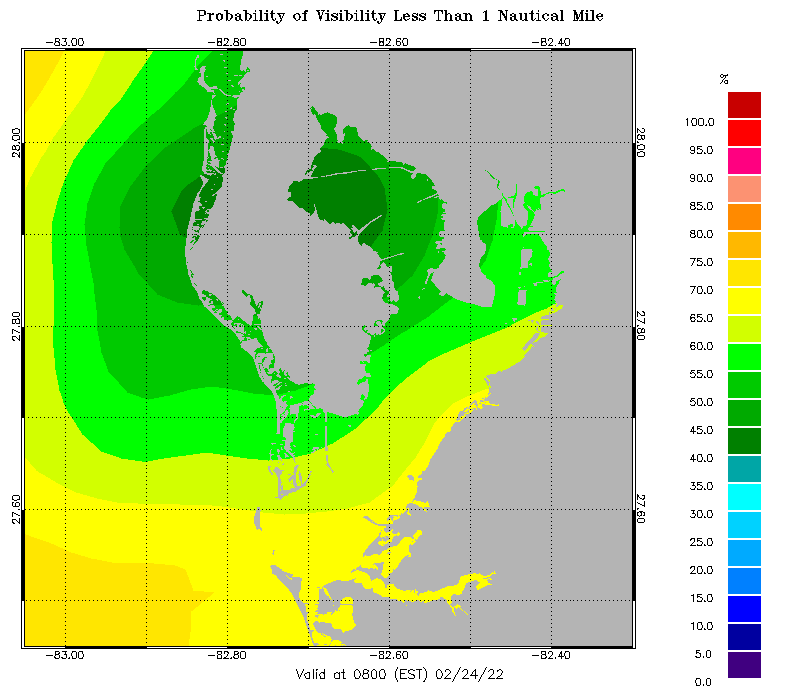
This website includes forecasts of visibility over Tampa Bay (and there are links to other coastal regions). The forecast below, for 1400 UTC 23 February / 0900 EST 23 February, has a maximum in predicted low visibility probability in about the right location. This forecast for the 24th suggests fog will be mostly offshore on the 25th.
Probability of low visibilities over/around Tampa Bay, valid 0900 EST on 24 February 2022 (Click to enlarge)
Low pressure just off the coast of South Carolina (0900 UTC map analysis) brought wide-spread fog and low ceilings to the southeastern United States on 7 February. The toggle below shows the Night Fog Brightness Temperature Difference (BTD, 10.3 µm – 3.9 µm) field that is often used to highlight regions where clouds made up of water droplets are widespread. The night time microphysics RGB includes as its green component the Night Fog BTD, and the correlation between the blue/cyan enhancement in the BTD and the cyan/yellowish color in the RGB is obvious. A challenge in using those two fields for low fog/stratus detection arises where multiple cloud layers might exist such that the BTD is not highlighting low cloud — because mid-level or high clouds block the satellite view of low clouds. This shortcoming is mitigated in IFR Probability fields by including information (from the Rapid Refresh model) on low-level saturation. Thus, IFR Probability fields suggest a greater likelihood for low clouds over coastal South Carolina (for example). If low-level saturation is *not* indicated in the model, IFR Probabilities will show minimal values, as over central Georgia (near Atlanta, especially), for example.
GOES-16 Night Fog Brightness Temperature Difference (10.3 µm – 3.9 µm), Night time microphysics RGB, and GOES-R IFR Probability, 1026 UTC on 7 February 2022 (Click to enlarge)
At 1156 UTC, a similar distribution to the three fields continues. Note how the presence of cirriform clouds over south-central Georgia affects the fields. The Night Fog BTD and Night Microphysics RGB both change radically, and IFR probabilities reduce — in part because the algorithm is less confident that low clouds exist. The small IFR Probabilities continue around Atlanta’s airline hub, important information from an aviation standpoint!
GOES-16 Night Fog Brightness Temperature Difference (10.3 µm – 3.9 µm), Night time microphysics RGB, and GOES-R IFR Probability, 1156 UTC on 7 February 2022 (Click to enlarge)
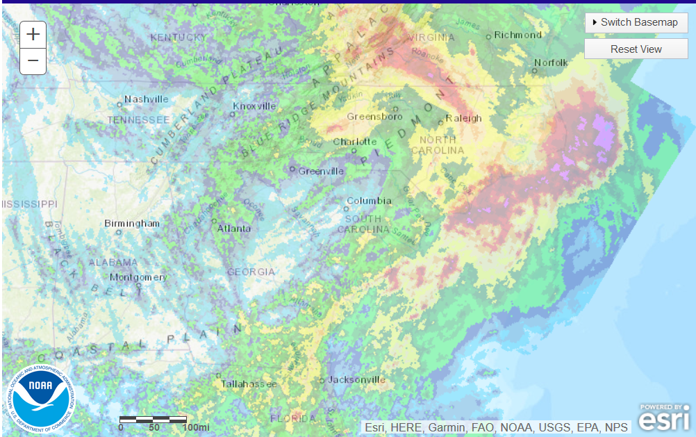
The toggle below compares IFR Probability with GOES-R Cloud Thickness. This is close to the time around sunrise/sunset when GOES-R Cloud Thickness are not computed because of quickly changing reflected solar shortwave infrared (3.9 µm) radiation; indeed, the cutoff can be viewed in the SSW-NNE terminator line over the Atlantic at the eastern edge of this image. If the low clouds on this day were strictly radiation (a dubious claim in the presence of rain!), then this scatterplot could be used to help decide when conditions might clear.
GOES-R IFR Probability and GOES-R Cloud Thickness fields, 1156 UTC on 7 February 2022 (Click to enlarge)
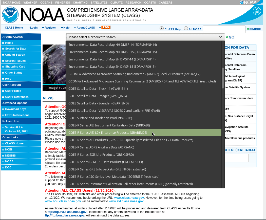
Starting 21 October 2021, GOES-R IFR Probability fields are archived (for both GOES-16 and GOES-17, Full Disk and CONUS/PACUS domains) at NOAA CLASS. These fields are available under the drop-down menu: Choose ‘GOES-R Series L2+ Enterprise Products (GRABINDE)’, as shown below.
Product Search drop-down menu from the landing page of NOAA CLASS
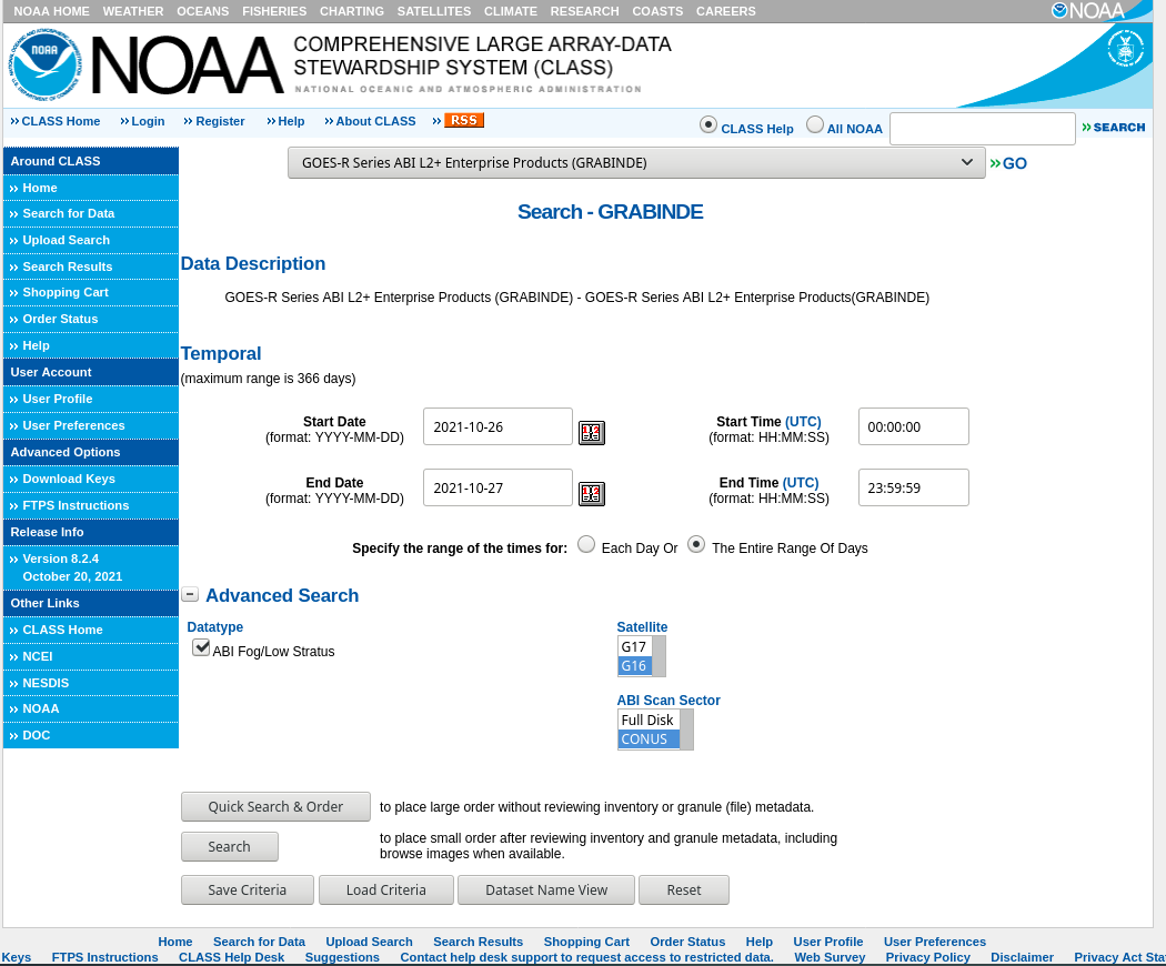
Clicking on ‘>>Go‘ after selecting the product takes a user to the page below, from which page ABI Fog/Low Stratus products can be obtained.
Product Selection page at NOAA CLASS for GOES-17/GOES-16 Fog/Low Stratus products (including Cloud Thickness and IFR Probability fields)
The files retrieved from CLASS will be netCDF files with a filename structure such as this:
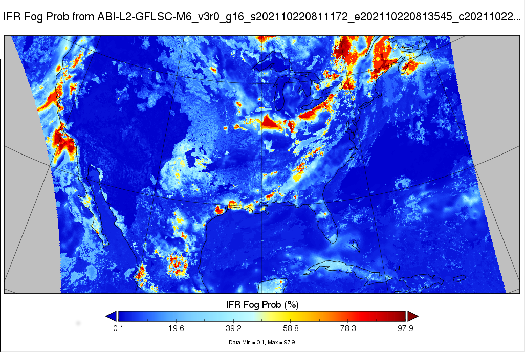
The file name above is for GOES-16 data from 0811 UTC on 22 October 2021. Such data can be displayed in (for example) Panoply, as shown below. Additionally, one could configure an AWIPS session to accept the fields.
IFR Probability fields, 0811 UTC on 22 October 2021 (GOES-16 CONUS) (Click to enlarge)
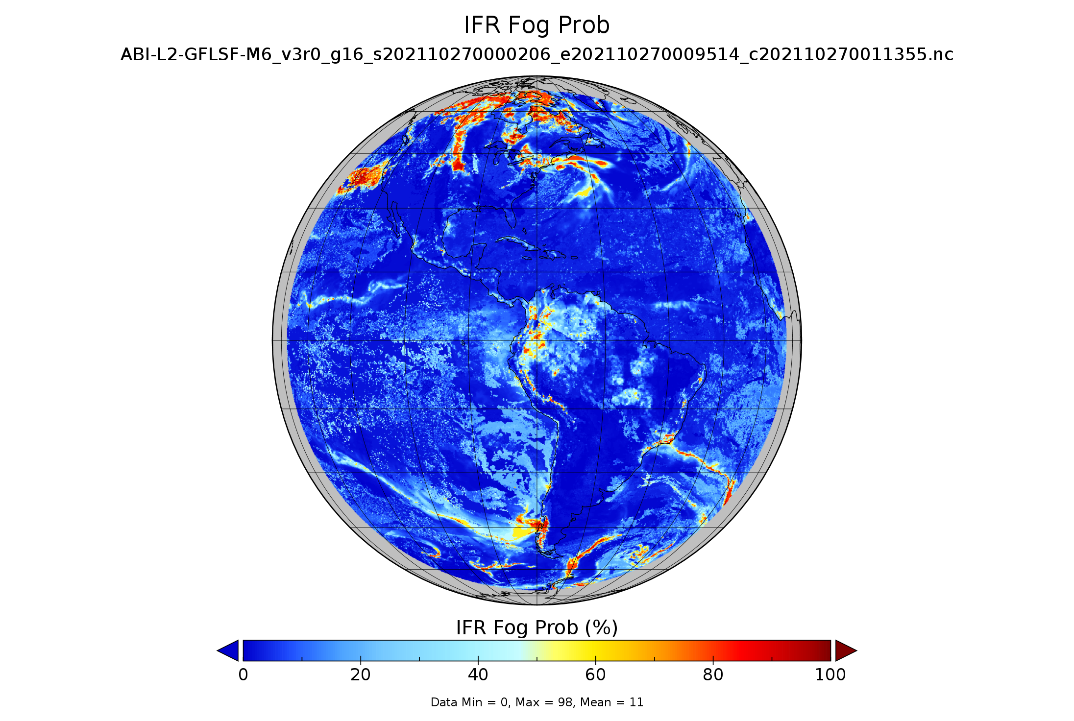
The netCDF files include many different 2-dimensional fields: IFR Probability, MVFR Probability, Low IFR Probability, Cloud Thickness, Maximum Relative Humidity between the surface and 500 feet AGL, Maximum Relative Humidity between the surface and 3000 feet AGL, Band 7 (3.9) Emissivitiy, and many more. A Full Disk image below (courtesy Tim Schmit, NOAA STAR), shows IFR Probability values on 27 October 2021 at 0000 UTC.
Global distribution of GOES-16 IFR Probability, 0000 UTC on 27 October 2021 (Click to enlarge)
GOES-16 IFR Probabilities (and surface observations of ceilings and visibilities), upper left ; GOES-16 Cloud Thickness, upper right ; GOES-16 ‘Night Fog’ Brightness Temperature Difference (10.3 µm – 3.9 µm), lower left; GOES-16 Nighttime Microphysics RGB, lower right. All from 0701 – 1301 UTC on 15 July 2021 (Click to enlarge)
The animation above shows various methods typically used to detect fog/low stratus in the early morning. Night Fog Brightness Temperature differences, bottom left, and Night Time microphysics, bottom right, are both satellite-only detection systems; a shortcoming might be that satellite data is challenged in detecting cloud bases — satellites view the cloud top. Additionally, the signal is lost as the sun rises. IFR Probability (upper right) includes information (from the Rapid Refresh model) on low-level saturation, so perhaps that field better defines the scattered pockets of fog apparent on this morning. However, the Rapid Refresh model resolution is 13-km, and a valley fog might not be well-resolved in the model.
The Cloud Thickness information suggests that any clouds are thin, and that morning burn-off will be speedy. That is indeed what happened, as shown by the 1500 UTC image below (taken from the CSPP Geosphere site). Recall that the Cloud Thickness product is not produced in the times that surround sunrise (or sunset).
CSPP Geosphere True Color image, 1500 UTC 15 July 2021 (Click to enlarge)
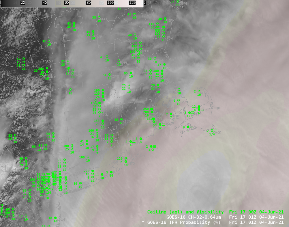
Toggle of GOES-16 visible Imagery (0.64 µm) and IFR Probability at 1701 UTC on 4 June 2021 (Click to enlarge). Surface observations of ceilings (AGL) and visibilities at 1700 UTC are included.
Mid-day observations over southeastern New England (and the offshore islands) show widespread fog. The toggle above shows mid-day visible imagery and GOES-16 IFR Probability. It’s very difficult to assess from the satellite imagery (especially on a day such as 4 June when high clouds are also present) alone where the reduced visibilities sit. Because IFR PRobability includes information on low-level saturation from the Rapid Refresh model, a better estimate of the horizontal extent of fog results. High IFR Probability values are widespread along the south coast of New England and the offshore islands where IFR and Low IFR conditions were observed. IFR Probability is a useful Situational Awareness tool. It can also be useful to load the imagery such that the IFR Probability is underneath a semi-transparent visible image, as shown below.
GOES-16 visible Imagery (0.64 µm) with underlain IFR Probability at 1701 UTC on 4 June 2021 (Click to enlarge). Surface observations of ceilings (AGL) and visibilities at 1700 UTC are included.
GOES-16 Brightness Temperature Difference (10.3 µm – 3.9 µm), 0831 – 1331 UTC 1 March 2021 (Click to enlarge)
GOES-16 Night Fog Brightness Temperature Difference (BTD) fields (10.3 µm – 3.9 µm), above, show different cloud types in and around South Carolina before and through sunrise on 1 March 2021. Before sunrises, low clouds — stratus and fog — are characterized by blue/cyan/aqua colors in this enhancement. The positive brightness temperature difference arises because of emissivity differences in small cloud droplets for shortwave (3.9 µm) and longwave (10.3 µm) infrared radiation. Negative brightness temperature differences occur for higher clouds.
The presence of high clouds interferes with the satellite’s ability to view low clouds. Although one can infer a low cloud’s presence from an animation (and the assumption that the cloud doesn’t substantively change when a high cloud overspreads it), it’s a bit more difficult to extrapolate the cloud base from the cloud top behavior. In other words: Are the low clouds highlighted actually fog? Note also how the BTD enhancement changes as reflected solar radiation around sunrise starts to overwhelm any differences attributable to emissivity.
IFR Probability fields, shown below, combine the strength of satellite detection of low clouds with the strength model depiction of low-level saturation. IFR Probabilities will be quite high where satellites detect low clouds, and where Rapid Refresh model simulations show near-surface saturation. But if high clouds are in the way, IFR Probabilities can still be large if the Rapid Refresh model shows low-level saturation. This is occurring off the coasts of South and North Carolina. Note also: IFR Probability fields aren’t changing radically as the sun rises.
GOES-16 IFR Probability, along with surface observations of ceilings and visibility, 0831 UTC – 1326 UTC 1 March 2021 (Click to enlarge)Night Fog Brightness Temperature Difference, Night time microphysics RGB, GOES-16 IFR Probability, 1001 UTC on 1 March 2021 (Click to enlarge)
The toggle above compares the Night Fog BTD with the Night time microphysics RGB (an RGB that takes as its green component the Night Fog BTD), and the GOES-16 IFR Probability fields at 1001 UTC on 1 March, shortly before sunrise. There is an obvious relationship between the RGB color and the regions of low clouds highlighted in the BTD by blue/cyan/aqua colors; the color of the RGB is tempered by the cloud temperature, however: the blue component of the RGB is the longwave infrared brightness temperature, and that is different over the ocean compared to over southwestern Georgia (for example). Note also how IFR Probability shows large values under the deep clouds over northwest South Carolina/western North Carolina.
Why is fog occurring offshore? Moist air over South Carolina is moving over relatively cool shelf waters, and cooled to its dewpoint; advection fog is the result. The toggle below shows surface dewpoints in the low 60s over coastal South Carolina. Sea-surface temperatures, shown at bottom from VIIRS at 0700 UTC and GOES-16 at 1300 UTC, show cool shelf waters with surface temperatures in the 50s (F).
GOES-16 IFR Probability with surface observations of ceilings/observations and surface METARs, 1001 UTC on 1 March 2021 (Click to enlarge)NOAA-20 ACSPO VIIRS Sea Surface Temperatures (0701 UTC) and GOES-16 SST Temperatures (1301 UTC), click to enlarge
GOES-16 versions of the GOES-R Fog/Low Stratus products are now available in Real Earth (see this post also). (The GOES-17 versions will become available when deemed operational). At present, only the CONUS domain is rendered into Real Earth. The animation below can also be accessed at this link.
GOES-16 IFR Probability, 1451 – 1516 UTC on 5 January 2021 (click to enlarge)
GOES-16 Visible Imagery, 1706 UTC on 9 September, with IFR Probability shown at the same time (with different alpha levels) (Click to enlarge)
GOES-R Fog/Low Stratus Products have been available in NWS Forecast Offices since 2012 via an LDM feed. GOES-16 versions for these products over the CONUS domain are now flowing over the Satellite Broadcast Network (SBN), effective 9 September 2020 (Announcement). Responsibility for this data feed is now at NESDIS following an extensive research-to-operations path. Fields distributed include Probability of: Marginal Visual Flight Rules (MVFR), Instrument Flight Rules (IFR) and Low Instrument Flight Rules (LIFR). In addition to these three probabilities (Click here to see an explanation), there is also a Low Cloud Thickness product that can be used to predict the dissipation time of radiation fogs.
IFR Probabilities, as shown above, are useful because they highlight regions under clouds where visibility restrictions are most likely. Loading it under a visible image and making the visible semi-transparent, as shown above, is a handy way to use the product. A forecaster responsible for transportation concerns can therefore focus their attention where it is needed, as defined by the IFR Probability field: IFR Probability is a good situational awareness tool.
Accessing the Fog/Low Stratus products via the SBN requires TOWR-S RPM v. 19 (It will be baselined in AWIPS v. 21.3.1 in 2021). GOES-17 (and GOES-16) IFR Probabilities are available at this website for the GOES-16 CONUS and GOES-17 PACUS sectors. Work is ongoing to product GOES-17 IFR Probabilities for Alaska.
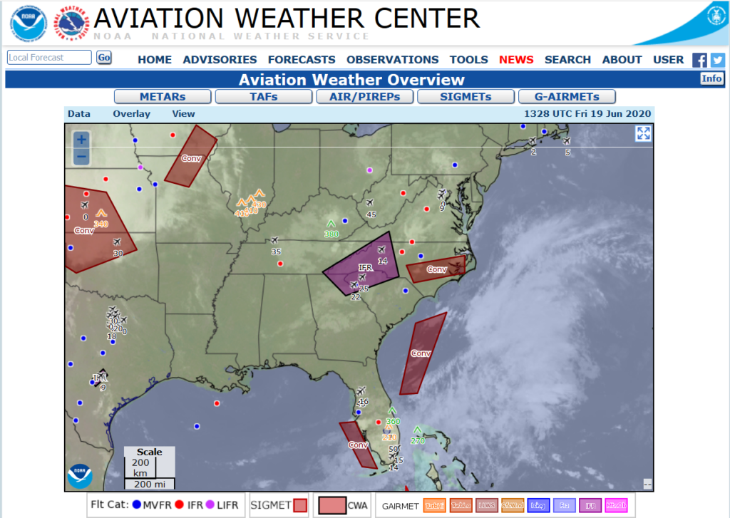
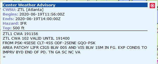
Fog developed over North and South Carolina (some of this region has been cloudy and wet for much of the past week; here is a weekly precipitation total from this site) on the morning of 19 June 2020; the screenshot above, from this site, shows a sigmet related to the IFR conditions present:
How did GOES-R IFR Probability capture this event? The animation below, from 0900 to 1306 UTC, shows generally high IFR Probabilities over most of the region. There are stations where IFR conditions are occurring and IFR Probabilities are low: the Columbus County Municipal Airport (KCPC, in southeast North Carolina), for example, shows obstructed ceilings and reduced visibility. This might be a localized sub-pixel scale fog related to the small streams near the airport there. A similarly small-scale fog event may be happening at Macon County airport (K1A5) in western North Carolina. The 0901 UTC Brightness Temperature Difference field shows a signal consistent with valley fog along the Little Tennessee River (see image at bottom)
Note how the signal shows little discernible impact from the rising of the Sun. A strength of this product is that uniformity — in contrast to the Night Fog Brightness Temperature difference field.
GOES-16 IFR Probabilities, 0901 UTC – 1306 UTC on 19 June 2020. Surface observations of ceilings and visibilities shown in blue (Click to enlarge)
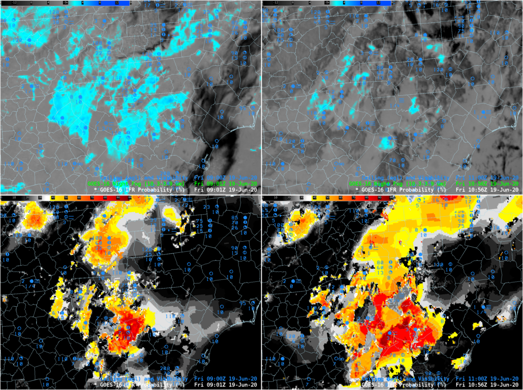
The 4-panel image below shows the ‘Night Fog’ Brightness Temperature Difference (10.3 µm – 3.9 µm, top) at 0901 and 1056 UTC and the IFR Probability fields, also at 0901 and 1056 UTC. IFR probability shows an expansion in the region of low ceilings reduced visibilities, as might be expected to occur around sunrise. The Night Fog Difference field shows a decrease in signal related to the increasing amount of reflected 3.9 µm solar insolation.
Night Fog Brightness Temperature Difference (10.3 µm – 3.9 µm), top and GOES-R IFR Probability, bottom, both at 0901 UTC (let) and 1056 UTC (right) on 19 June 2020.
GOES-16 ABI Band 02 (0.64 mm “Red Visible”) visible imagery, 1201-2311 UTC on 20 April 2020
GOES_16 Visible imagery, above (along with surface observations of ceilings and visibilities), shows fog and low clouds over south Texas and offshore waters. The observations plotted can allow you to determine where IFR conditions are apparent — where visibilities are between 1 and 3 statute miles and ceilings are between 500 and 1000 feet. It’s difficult to determine the area of IFR conditions based solely on cloud cover however.
The animation below shows the probability of IFR conditions, a product that fuses satellite information with low-level saturation information from the Rapid Refresh model (Click here for an animation with no observations). The morning fog over east Texas burns off fairly quickly, and only dense sea fog is left after about 1700 UTC (10 AM CDT). In many offshore regions (and over east Texas before sunrise), the IFR Probability field has a flat character to it that is typical of a IFR Probability field determined mostly by model data. More pixelated data (and somewhat higher probabilities) occur where breaks in the cloud allow for satellite data to identify low clouds.
GOES-R IFR Probability, 1101 UTC to 2311 UTC on 20 April 2020
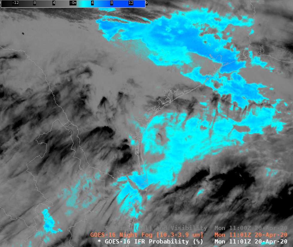
The night fog brightness temperature difference field, below, highlights a challenge in identifying low clouds using satellite data alone (in contrast to the IFR Probability above that uses satellite and model data, fusing the strengths of both). When cirrus is present, it can mask the satellite’s view of the low cloud beneath. In addition, the Night Fog Brightness Temperature difference product is not consistent through sunrise, as the emissivity differences that drive the signal at night time (small cloud droplets are not black body emitters of 3.9 µm radiation, but they are blackbody emitters of 10.3 µm radiation) become overwhelmed by reflectivity differences during the day when far more 3.9 µm solar radiation is reflected than 10.3 µm solar radiation. Thus, in the day, both low clouds and high clouds show up as black in this enhancement: they are both able reflectors of 3.9 µm radiation.
Night Fog Brightness Temperature Difference (10.3 µm – 3.9 µm) fields from 1101 UTC to 2311 UTC on 20 April 2020
The Day Fog Brightness Temperature Difference field, below, shows how cirrus ice crystals are initially more reflective of solar radiation, but as the sun climbs higher in the sky, low clouds start to reflect just as much solar radiation.
Day Fog Brightness Temperature Difference (3.9 µm – 10.3 µm) fields from 1201 UTC to 2311 UTC on 20 April 2020GOES-16 Night Fog Brightness Temperature Difference (10.3 µm – 3.9 µm), 1101 UTC on 20 April 2020
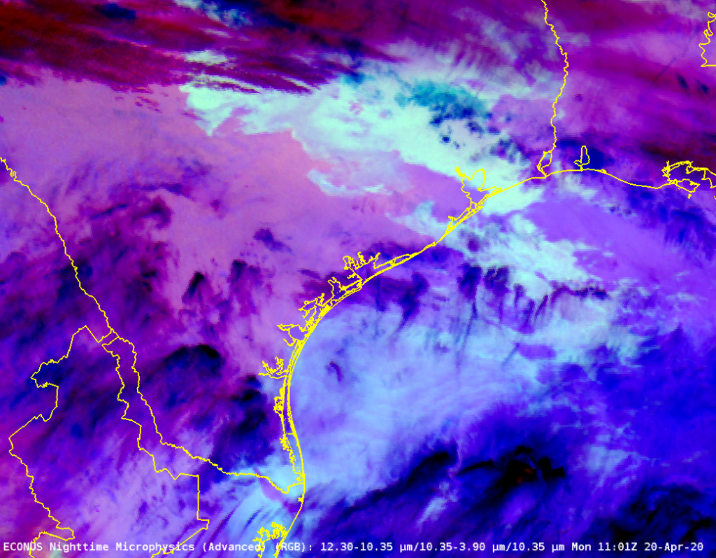
The Night Fog Brightness Temperature Difference field, above, is a key component (the ‘green’ part) of the Advanced Night Time Microphysics RGB, shown below. Where the Brightness Temperature Difference field is unable to view low clouds, similarly the Night Time Microphysics RGB will be unable to highlight them.
GOES_16 Night Fog Microphysics, 1101 UTC 20 April 2020
Thanks to Penny Harness, WFO Corpus Christi, for alerting us to this event. (Link)


