Monthly Archives: November 2013

A Reminder about Co-Registration Errors

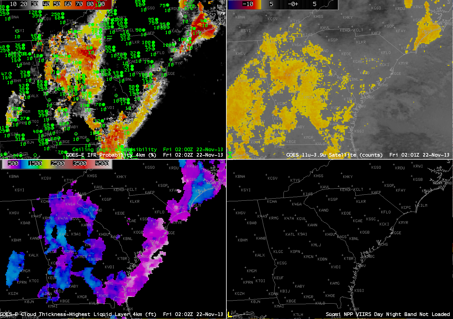
GOES-R IFR Probabilities from GOES-13, times as indicated on 27 November 2013 (click image to enlarge)

The GOES-R IFR Probability field showed enhanced probabilities surrounding lakes and rivers in Louisiana and Texas overnight. This is in large part due to a strong signal in the Brightness Temperature Difference field. There is a co-registration error between the 10.7 µm and 3.9 µm detectors on the GOES Imager. This means that the pixel locations for the two channels are not aligned, and at times the mis-alignment is large enough that a fog signal is produced. In the present case, one of the detectors sees the warm waters of a lake, and the second detector sees the adjacent (much cooler) shoreline, but the navigation misalignment is such that both pixels are believed to be co-located. Thus a difference in the brightness temperature occurs not because of emissivity difference properties in clouds (which also makes the 3.9 micron brightness temperature appear cooler) but because of a co-registration error. The brightness temperature difference field from 0802 UTC is below (the 0745 UTC image is very similar). Note how the enhanced brightness temperature difference field appears to have a shadow just to its west. It is possible for this to occur if a cloud is forming downwind of a warm lake. However, in the present case, winds were primarily northerly, not westerly.

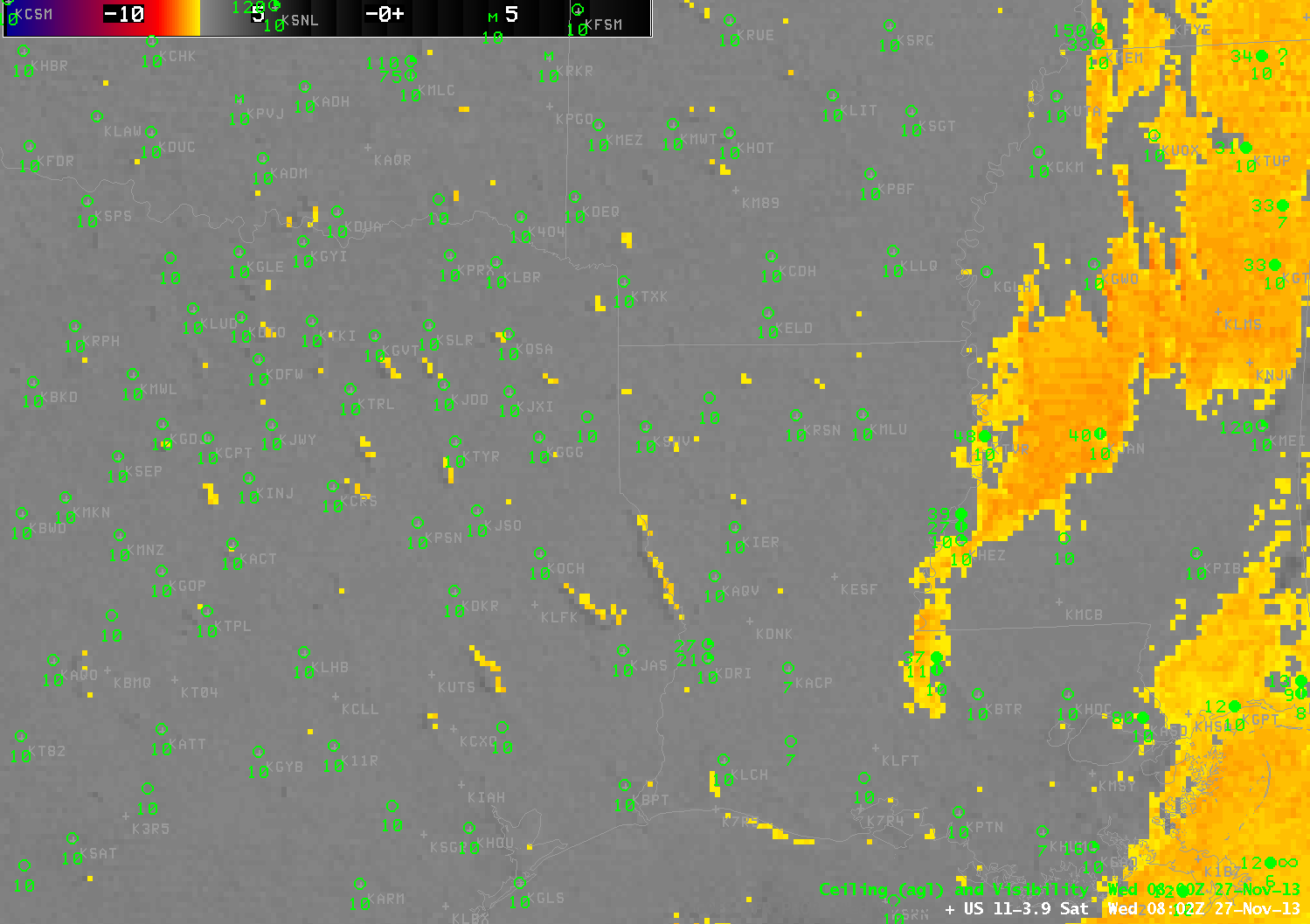
GOES-13 Brightness Temperature Difference Product (10.7 µm – 3.9 µm) 0802 UTC 27 November 2013 (click image to enlarge)

Polar Orbiting satellites viewed this region contemporaneously. Aqua, carrying the MODIS instrument, passed overhead at 0745 UTC, and Suomi/NPP at 0802. What did they see? The 3.9 µm channel from MODIS, below, highlights the warm lake waters over eastern Texas and Louisiana. There is little indication in this image of clouds near the lakes.

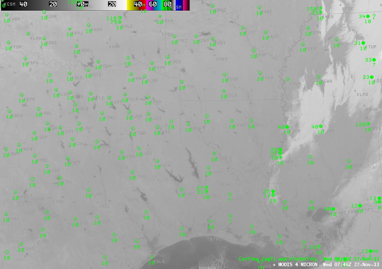
MODIS Brightness temperature at ~3.9 µm 0802 UTC 27 November 2013 (click image to enlarge)

The brightness temperature difference product from MODIS, below, and the MODIS-based IFR Probabilities also show no indication of fog/low stratus near the bodies of water in east Texas/Louisiana.

MODIS Brightness temperature difference (11.0 µm – 3.9 µm) and MODIS-based IFR Probabilities at 0746 UTC 27 November 2013 (click image to enlarge)

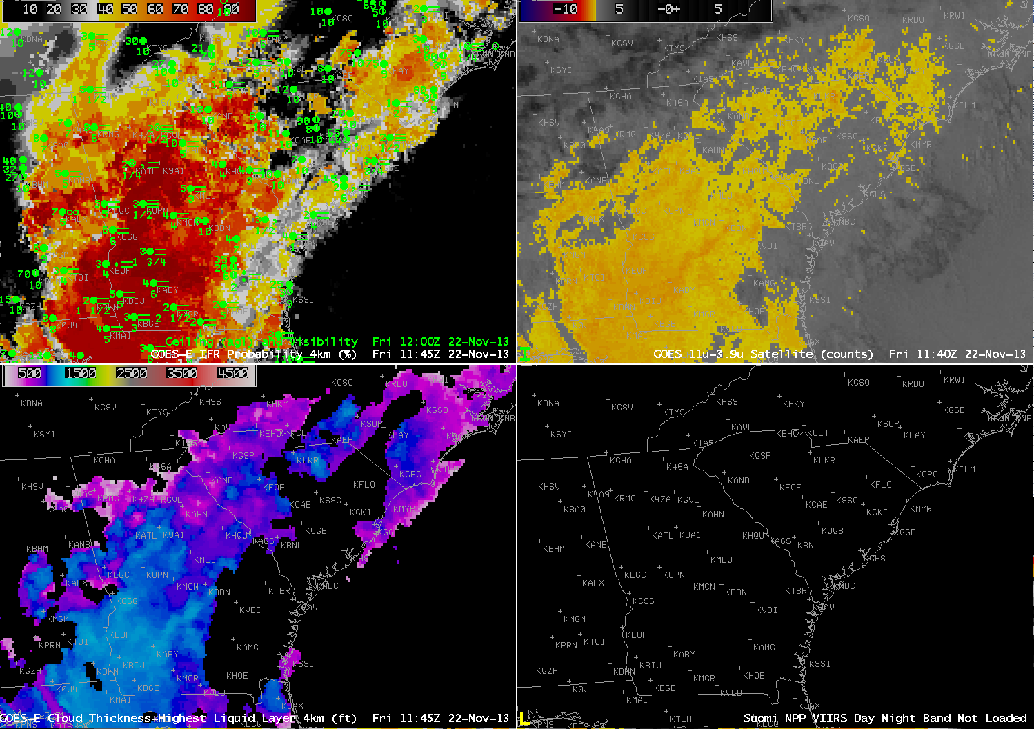
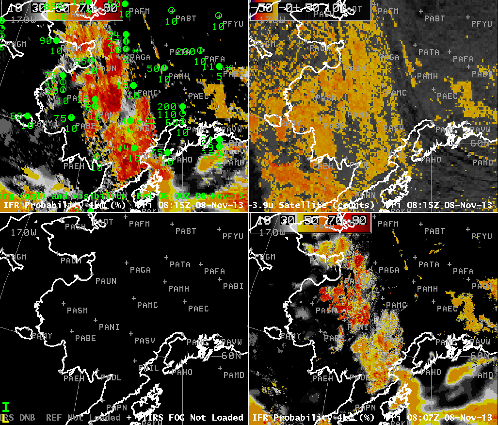
Suomi/NPP data are shown below. The Brightness Temperature Difference (10.35 µm – 3.74 µm) Field, the 3.74 µm field and the Day/Night band all are consistent with clear skies near the water bodies of east Texas and western Louisiana.

Suomi/NPP VIIRS Brightness Temperature Difference (10.35 µm – 3.74 µm) and Day/Night band at 0802 UTC 27 November 2013 (click image to enlarge)

Be cautious when interpreting the brightness temperature difference from GOES (and IFR Probabilities that are computed using the satellite signal) along land/water boundaries. GOES Engineers continue to investigate methods of mitigating this co-registration error.

Fog and Stratus in the Southeast United States

Fog and Stratus with IFR Conditions developed along the Southeast Coast of the United States on the morning of November 22. In some places, the GOES-IFR Probability fields gave a signal of the developing visibility obstructions more than an hour before the traditional brightness temperature difference signal. At 0202 UTC, below, the IFR Probability fields suggest a continuous region of enhanced probabilities of IFR conditions developing along the South Carolina coastline. Both IFR Probabilities and the brightness temperature difference fields agree that Fog/Low Stratus are already present over coastal North Carolina.

GOES-R IFR Probabilities from GOES-13 (Upper Left), GOES-13 Brightness Temperature Difference Product (10.7 µm – 3.9 µm) (Upper Right), GOES-R Cloud Thickness from GOES-13 (Lower Left), Suomi/NPP Day/Night Band (Lower Right), at 0202 UTC 22 November 2013 (click image to enlarge)

At 0315 UTC, IFR Probabilities continue to increase along the South Carolina coast. In contrast, Brightness Temperature difference fields are showing less of a signal suggestive of fog and low stratus. There was a Terra overpass at 0316 UTC that allowed MODIS data to be used in the GOES-R IFR Probability algorithm, and that field agrees well with the GOES-based field.

GOES-R IFR Probabilities from GOES-13 (Upper Left), GOES-13 Brightness Temperature Difference Product (10.7 µm – 3.9 µm) (Upper Right), GOES-R Cloud Thickness from GOES-13 (Lower Left), GOES-R IFR Probabilities computed from MODIS data (Lower Right), at ~0315 UTC 22 November 2013 (click image to enlarge)

At 0502 UTC, GOES-R IFR Probabilities are still high in a narrow corridor along the coast, despite the lack of a distinct signal from GOES-East in the brightness temperature difference field.

At 0615 UTC, the brightness temperature difference field starts to show a signal that is consistent with the presence of fog and low stratus along coastal South Carolina. GOES-R IFR Probabilities increase, as well. This is to be expected because the GOES-R algorithms use signals from both the GOES Satellite and the Rapid Refresh data to compute IFR Probabilities. Given that the Rapid Refresh data has been suggesting Fog/Low Stratus might be present (something that can be assumed to be true given the elevated probabilities that could alert any forecaster to the presence of developing fog that have been present for hours in the absence of a distinct signal from satellite), the appearance of a definitive satellite signal should only increase the probability of IFR conditions. At 0616, Suomi/NPP was viewing coastal South Carolina, and both the Day/Night band and the brightness temperature field are shown in the figure below. GOES-R IFR Probability algorithms do not yet incorporate Suomi/NPP data.

GOES-R IFR Probabilities from GOES-13 (Upper Left), GOES-13 Brightness Temperature Difference Product (10.7 µm – 3.9 µm) (Upper Right), GOES-R Cloud Thickness from GOES-13 (Lower Left), Toggle between Suomi/NPP Day/Night Band and Brightness Temperature Difference (Lower Right), at ~0615 UTC 22 November 2013 (click image to enlarge)

By 0800 UTC, below, IFR Conditions are reported at Charleston, SC, and GOES-R IFR Probabilities, brightness temperature difference field from GOES and Suomi/NPP and the Day/Night Band from Suomi/NPP all suggest the presence of fog/low stratus. To the northwest, over southeastern Tennessee, high clouds are obscuring the satellite view of any stratus/fog that is present (IFR Conditions are reported at, for example, Crossville, TN).

GOES-R IFR Probabilities from GOES-13 (Upper Left), GOES-13 Brightness Temperature Difference Product (10.7 µm – 3.9 µm) (Upper Right), GOES-R Cloud Thickness from GOES-13 (Lower Left), Toggle between Suomi/NPP Day/Night Band and Brightness Temperature Difference (Lower Right), at ~0800 UTC 22 November 2013 (click image to enlarge)

At 1145 UTC, IFR Probabilities maintain their high values along coastal South Carolina (and all of southwest Georgia) where IFR conditions are occurring. Note how the GOES-13 Brightness temperature difference product has highlighted values over central South Carolina, where IFR conditions are not reported. In this region, the Rapid Refresh model data is not showing saturation (or near-saturation) consistent with low-level stratus/fog so IFR Probabilities are reduced.

1145 UTC is the last image for GOES-R Cloud Thickness prior to twilight conditions. Data in the image can be used (in concert with this chart) to predict the dissipation time for radiation fog. GOES-R Cloud Thickness values over southeast Georgia range from 950 to 1100 feet, suggesting a dissipation time of 3 hours, or near 1445 UTC.

(Added: Later in the day)

Higher clouds allowed the low clouds to linger. By 1732 UTC, the low clouds had almost dissipated.

GOES-13 Visible Imagery, 1732 UTC 22 November 2013 (click image to enlarge)

Fog in eastern Washington

GOES-15-based GOES-R IFR Probabilities (Upper Left), GOES-15 Brightness Temperature Difference Product (10.7 µm – 3.9 µm) (Upper Right), GOES-R Cloud Thickness from GOES-15 (Lower Left), Suomi/NPP Brightness Temperature Difference and GOES-15 Visible data (Lower Right), all times as indicated (click image to enlarge)

The evolution of GOES-R IFR Probability fields showed an expected relationship between where Fog and Low stratus caused IFR Conditions and where IFR Probability was highest. The hourly animation, above, shows very high IFR Probabilities in and around Spokane in concert with IFR conditions that are observed. The Brightness Temperature Difference product, upper right, shows a strong signal there as well, but the positive signal extends to regions where IFR conditions are not observed: for example, over western Montana near Missoula. GOES-R IFR Probability fields thus are refining the signal in the brightness temperature difference field; the Rapid Refresh Model output allows the IFR Probability field algorithm to distinguish between fog/low stratus and mid-level stratus.

Later in the animation, IFR Probabilities decrease around Spokane as high-level clouds move in. Because these high clouds obscure the satellite view of low- and mid-level clouds, satellite information is not included in the computation of IFR Probabilities and Probabilities are lower. At the end of the animation, during the day, probabilities increase. Use of the visible data as a cloud-clearing product leads to higher probabilities (because there is more confidence that the cloud is actually present).

Note that Cloud Thickness is only computed in regions of low clouds that are comprised of water droplets. When high clouds are present, cloud thickness is not computed. In addition, cloud thickness is not computed during twilight conditions on either side of sunrise and sunset. Those restrictions show up plainly in the cloud thickness field in the animation.

How accurate are GOES-R Cloud Thickness Fields?

GOES-13-based GOES-R IFR Probabilities (Upper Left), GOES-13 Brightness Temperature Difference Product (10.7 µm – 3.9 µm) (Upper Right), GOES-R Cloud Thickness from GOES-East (Lower Left), GOES-R Cloud Thickness from GOES-West (Lower Right), all times as indicated (click image to enlarge)

GOES-R IFR Probabilities over the Central Plains from just before sunrise on 11 November 2013 are displayed above. The IFR Probabilities accurately depict the region of lower stratus and fog with reduced visibilities, separating that region from the mid-level stratus over eastern Kansas and western Missouri. In contrast the brightness temperature difference field (10.7 µm – 3.9 µm) highlights the entire region as one of interest.

The GOES-R Cloud Thickness from GOES-East (bottom left) and from GOES-West (bottom right) show cloud thickness over Dodge City at just under 1200 feet. Note that the values computed with GOES-West are somewhat larger because of the oblique view angle from GOES-West. The 1200 UTC sounding from Dodge City, below, shows a fog/stratus deck from the surface (928 mb, 2652 feet ASL) to 880 mb (4075 feet ASL), a thickness of 1423 feet. Given that the sounding is not saturated at the surface, that 1423 foot thickness is likely a slight overestimate. It is very close to the GOES-R Cloud Thickness estimate of 1200 feet, however.

1200 UTC Sounding at Dodge City, Kansas, 11 November 2013 (click image to enlarge)

Fog/Low Stratus over southwest Alaska on November 8

GOES-15-based GOES-R IFR Probabilities every half hour from 0300 UTC through 1530 UTC (click image to animate)

Fog and low stratus were present over southwestern Alaska early on November 8. How did the GOES-R IFR Probability fields perform compared to the heritage brightness temperature difference (in this case, 10.7 µm – 3.9 µm from GOES-15). Consider the airport PARS (southwest of Anvik — PANV and northwest of Aniak — PANI). IFR conditions are present there until 0900 UTC, when ceilings rise and IFR probabilities drop. Subsequently, IFR Probabilities increase again as a north-south oriented region of higher IFR probabilities moves over, and IFR conditions are again present by 1600 UTC. Further south, PAJZ and PAIG report IFR conditions when IFR Probabilities are high, and conditions improve as IFR Probabilities decrease. IFR Probabilities initially around PAIG have the characteristic flat field (and somewhat lower probability) associated with a region where high-level clouds are present. In these regions, only Rapid Refresh data can be used to compute the probability; because satellite predictors are not used, the computed IFR probabilities are lower.

Compare the IFR Probability field, above, to the Brightness Temperature Difference field, below, that has been color-enhanced to highlight regions where water-based clouds may be present. The IFR Probability field correctly reduces the regions where IFR conditions might be occurring. That is, the traditional brightness temperature difference field is plagued by many false positives. This is because mid-level stratus that is unimportant for transportation looks to a satellite to be very similar to low-level stratus that is important for transportation.

GOES-15 Brightness Temperature Difference (10.7 µm – 3.9 µm) every hour from 0300 UTC through 1500 UTC (click image to animate)

MODIS data from the polar-orbiting satellites Terra and Aqua can also be used to compute IFR Probabilities, and MODIS data — although less frequent than the data from the geostationary GOES-15 — has far superior horizontal resolution (nominal MODIS resolution is 1 km at nadir) to GOES data (nominally 4 km at the sub-satellite point over the Equator) over Alaska. Small-scale features are much more likely to be detected in MODIS data, as shown below.

GOES-15-based GOES-R IFR Probabilities (Upper Left), GOES-15 Brightness Temperature Difference Product (10.7 µm – 3.9 µm) (Upper Right), Suomi-NPP Brightness Temperature Difference (11.45 µm – 3.74 µm) and Day/Night band (Lower Left), MODIS-based GOES-R IFR Probabilities (Lower Right), all times as indicated (click image to enlarge)

The Day/Night band from Suomi/NPP can sometimes be used to detect cloud features. However, when the Moon is not present to provide illumination, cloud detection is a challenge. In the toggle above between the Day/Night band and the brightness temperature difference from VIIRS (11.45 – 3.74), for example, there is little evidence of the apparent cloud edge that is visible both in VIIRS data, in GOES-15 data (Upper right) and in the IFR Probability fields from GOES (Upper Left) and MODIS (Lower Right).

Fog and Stratus in one scene: What should be highlighted?

GOES-13-based GOES-R IFR Probabilities (Upper Left), GOES-13 Brightness Temperature Difference Product (10.7 µm – 3.9 µm) (Upper Right), GOES-R Cloud Thickness (Lower Left), Suomi-NPP Day/Night band (Lower Right), all times as indicated (click image to enlarge)

Dense fog developed over Western Wisconsin before sunrise on 5 November 2013. The animation above shows the development of high IFR probabilities in that region as a mid-level stratus deck shifts off to the east. Cloud thicknesses just before sunrise reach 1100 feet over portions of Wisconsin; according to this plot, fog should persist for at least 4 hours after sunrise. This was the case. Fog dissipated shortly after 1700 UTC.

This case shows a benefit of the GOES-R IFR Probability field: it accurately discerns the difference between low stratus/fog (that develops over western Wisconsin) and mid-level stratus (retreating to the east over central and eastern Wisconsin during the animation). Mid-level stratus is normally not a transportation concern whereas low clouds/fog most definitely are; in this case, dense fog advisories were issued by the Lacrosse, WI, WFO (ARX). At the beginning of the animation, widespread mid-level stratus is indicated (IFR conditions are not reported). As the night progresses, IFR Probabilities increase in regions where IFR conditions start to be reported. (A brightness temperature signal in GOES also develops in this region).

As above, but at 0815 UTC. The lower right image toggles between the Day/Night Band and the Brightness Temperature Difference (11.45 µm – 3.74 µm) from Suomi/NPP (click image to enlarge)

Suomi/NPP VIIRS viewed this scene shortly after 0815 UTC, and that imagery is above. Both the Day/Night band and the Brightness Temperature Difference fields (11.45 µm – 3.74 µm) are shown as a toggle. The mid-level stratus at 0815 is readily apparent. The developing fog over river valleys in western Wisconsin shows plainly in the brightness temperature difference field, but less so in the day/night band with scant lunar illumination.

GOES-13-based GOES-R IFR Probabilities (Upper Left), GOES-13 Brightness Temperature Difference Product (10.7 µm – 3.9 µm) (Upper Right), GOES-R Cloud Thickness (Lower Left), MODIS-based IFR Probabilities (Lower Right), all times as indicated (click image to animate)

MODIS data from Terra and Aqua is also used to produce IFR Probabilities, and those data are shown above, for three times: 0413 UTC, 0823 UTC and 1609 UTC. Patterns in the MODIS IFR Probability are similar to those in GOES, but small-scale features such as river valleys are much more apparent. Note that by 1609 UTC, higher clouds have overspread western Wisconsin in advance of an approaching mid-latitude cyclone; thus, the GOES and MODIS IFR Probabilities both are flat fields that are mostly based on Rapid Refresh data. Nevertheless, they both depict the region of IFR conditions over western Wisconsin that is surrounded by better visibilities and higher ceilings. Recall that GOES-R cloud thickness is not computed where high clouds are present.

GOES-R Fog Product Examples

Fog detection fusing GOES, Terra/Aqua or Suomi/NPP Satellite data with Model output