Category Archives: Wisconsin

River Fog over Wisconsin

GOES-16 IFR Probability, 0747-1152 UTC on 30 August 2018 (Click to enlarge)

GOES-16 IFR Probability incorporates information about low-level saturation from the Rapid Refresh Model. The model data used changes hourly, and that can cause an hourly change, a pulsing, in the IFR Probability animation in cases when the forecast model evolution is changing.

In this case, visible imagery at sunrise (enhanced because of the low light) suggests the IFR Probability field is overpredicting the extent of River Fog in southwest Wisconsin. Note, however, that the highest IFR Probabilities do align with river valleys where fog is observed.

GOES-16 ABI Band 2 (0.64 µm) and GOES-R IFR Probabiilty, 1152 UTC on 30 August 2018 (Click to enlarge)

Dense Fog over the Midwestern United States

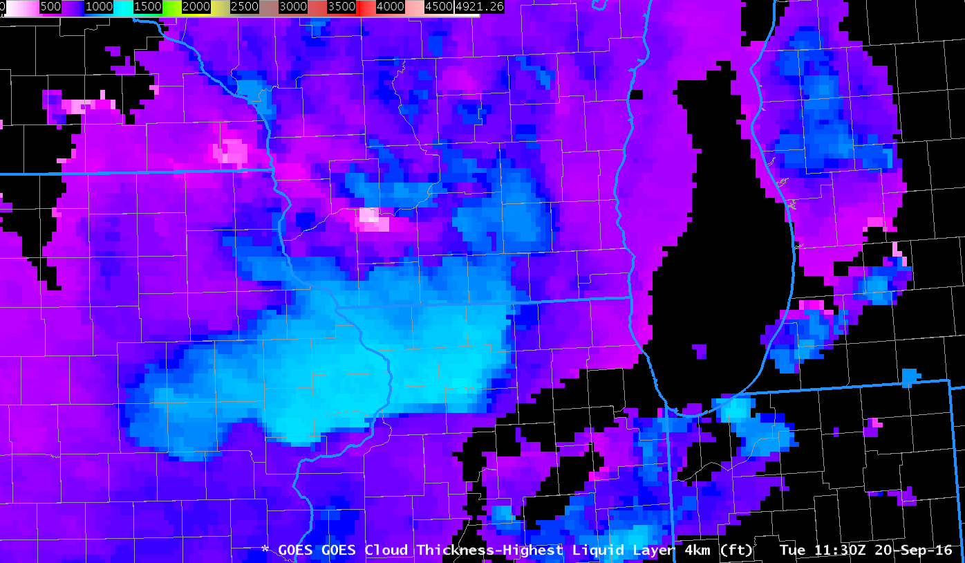
GOES-R IFR Probability Fields, 0337 – 1332 UTC on 8 August 2018 (Click to enlarge)

The longer August nights over the upper Midwest (for example, Madison Wisconsin’s night is about 70 minutes longer now than it was at the Summer Solstice) can allow for dense fog to form when light winds and clear skies follow a cloudy, damp day. The animation above shows the evolution of the GOES-R IFR Probability fields as the dense fog develops, a fog for which advisories were issued. The horizontal extent of the widespread fog is captured well in the IFR Probability fields. There are a couple of things worth noting.

There is a subtle — but noticeable — change in the IFR Probability Fields each hour in the animation. That change is related to model data in this fused product. Rapid Refresh Model output are used to identify regions of low-level saturation that must occur with fog. (The inclusion of this data helps IFR Probability better distinguish — compared to satellite imagery alone — between elevated stratus and fog). When output from newer model runs is incorporated (and that happens every hour), the IFR probability fields are affected. The amount of change is testimony to whether the sequential runs of the Rapid Refresh are consistent in capturing the developing fog. In this case, there were differences from one model run to the next.

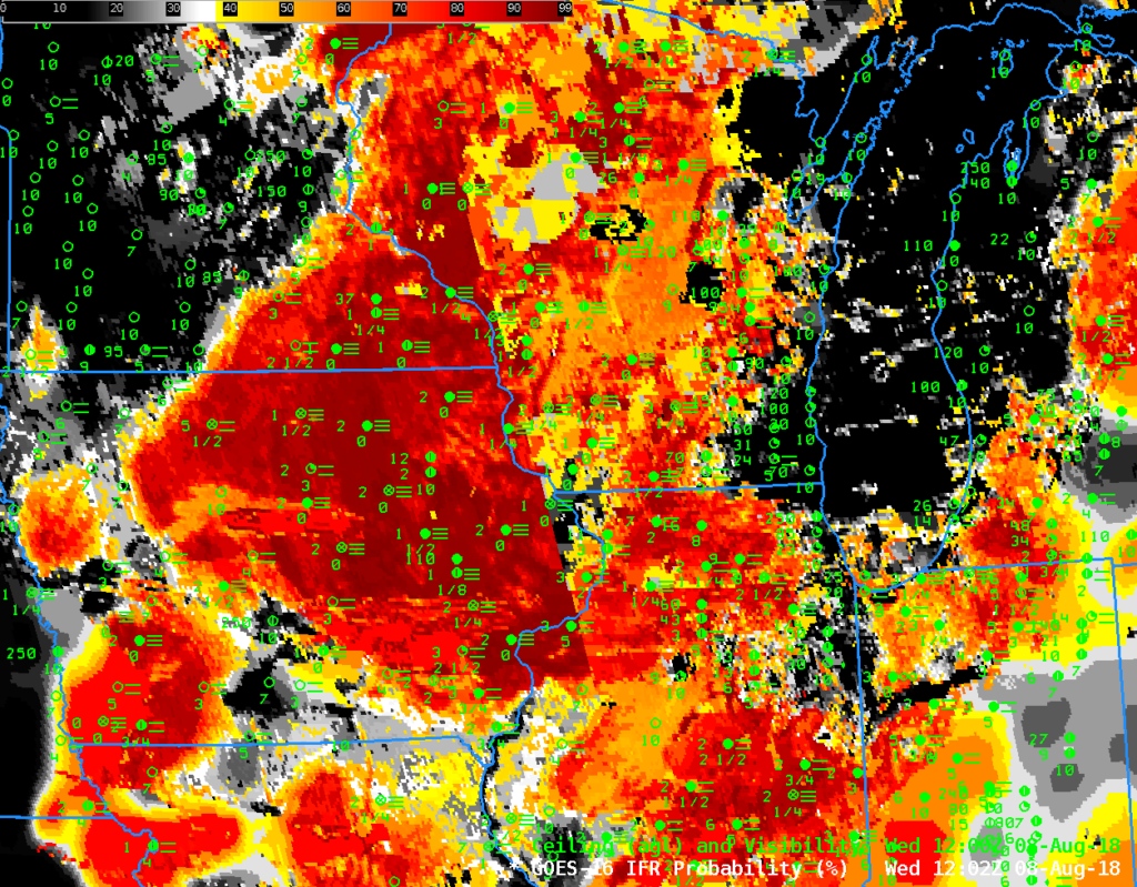
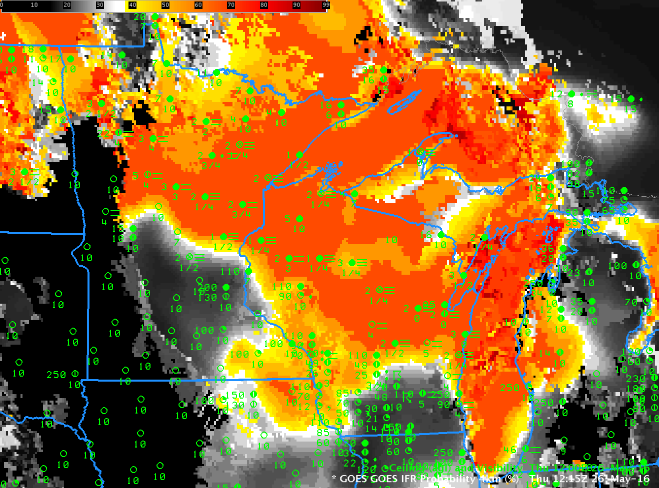
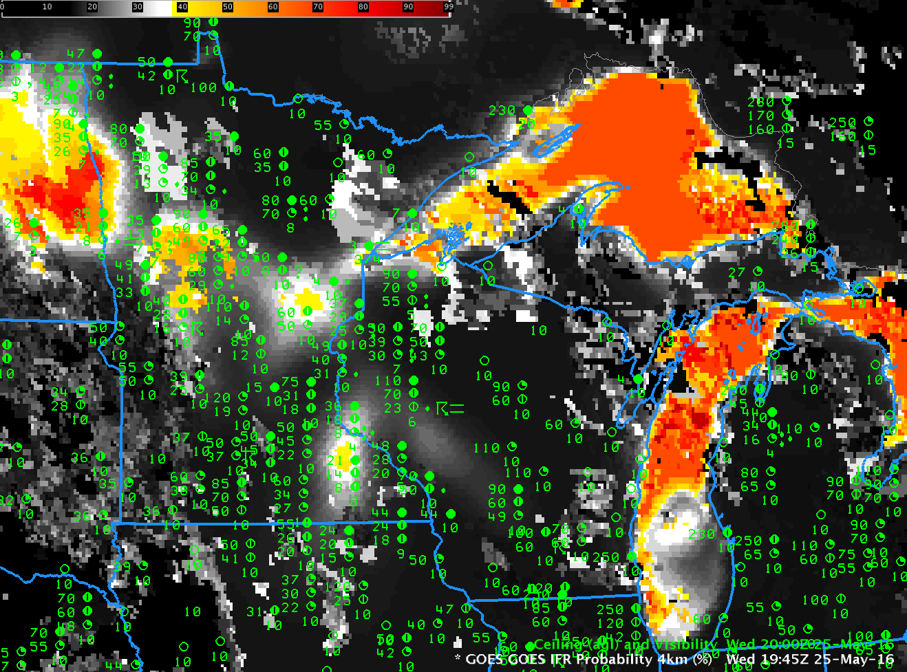
GOES-R IFR Probability fields, 1202 UTC on 8 August 2018 (Click to enlarge)

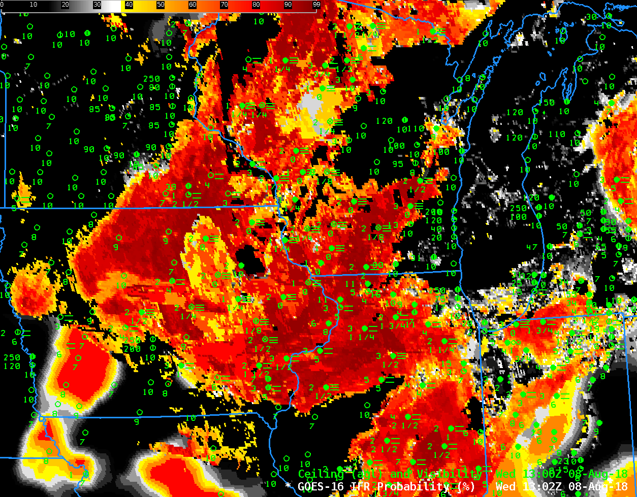
Two boundaries are apparent in the animation above, captured in the 1202 UTC image above, and in the 1302 UTC image below. These boundaries are related to the Terminator, the dividing line between night and day. During an hour around sunrise, rapid changes in reflected 3.9 µm solar radiation make the detection of low clouds difficult. Temporal adjustments are incorporated into the IFR Probability fields to create a cleaner field. In the 1202 UTC image, above, the effects of sunrise are occurring along the NNW-SSE oriented boundary near the Mississippi River in southwestern WI (The boundary is parallel to the Terminator line, so it will be vertical — parallel to a Longitudinal Line — on the Equinoxes). In the 1302 UTC image, below, the second boundary is over far northwestern Wisconsin, far southeastern Minnesota, and eastern Iowa. The region between these two westward-propagating boundaries is where information from previous times is used in the IFR Probability fields. Thus, when the second boundary passes, you may observe rapid changes in IFR Probability fields.

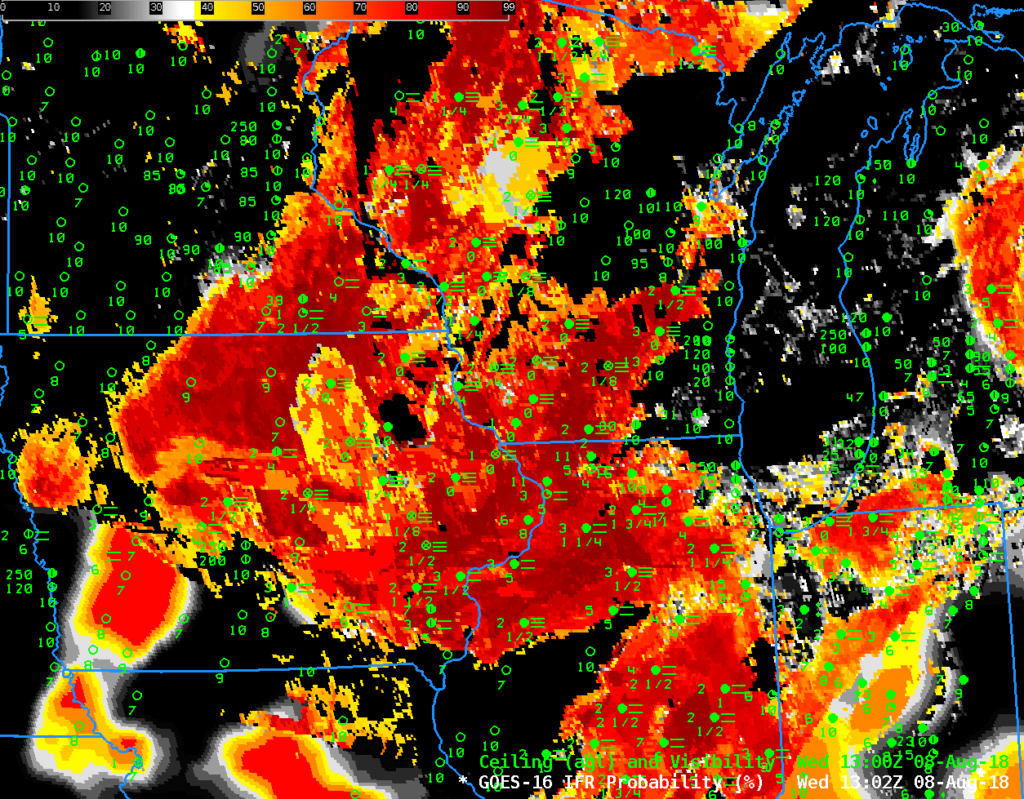
GOES-R IFR Probability fields, 1302 UTC on 8 August 2018 (Click to enlarge)

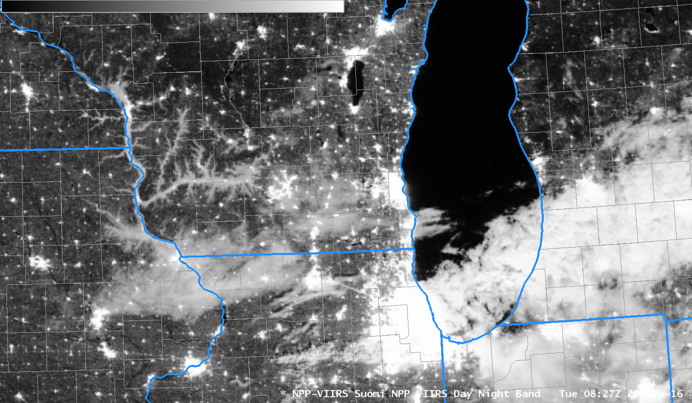
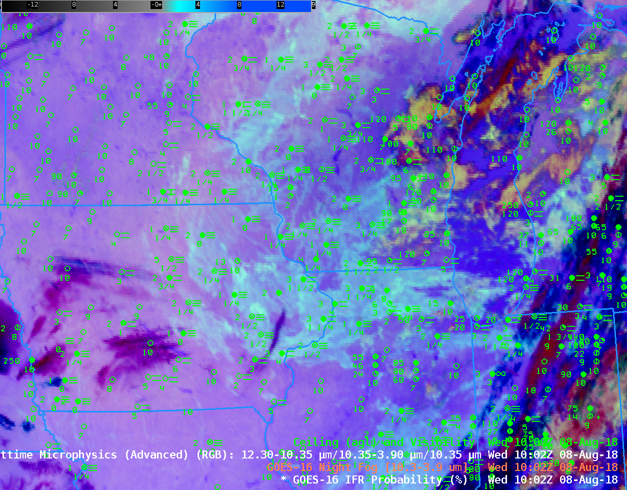
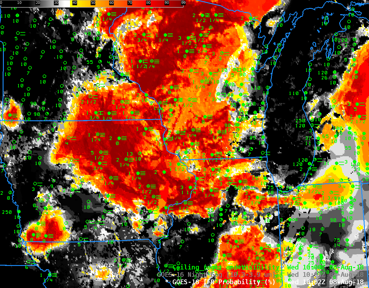
The Night Fog Brightness Temperature Difference (10.3 µm – 3.9 µm) can be used to detect stratus, and that field is also a constituent (the ‘green’ part) of the Advanced Nighttime Microphysics RGB. The animation below compares these two products used to detect stratus with IFR Probability at 1002 UTC on 8 August 2018. The Night Fog Brightness Temperature Difference fails to highlight regions of fog over central WI (and elsewhere), so neither it nor the RGB give a consistent signal over the entire fog-shrouded region.

Night Fog Brightness Temperature Difference (10.3 µm – 3.9 µm), GOES-R IFR Probability, and Advanced Nighttime Microphysics RGB at 1002 UTC on 8 August 2018 (Click to enlarge)

IFR Probability indicating a Cold Front

GOES-16 IFR Probability Fields, 0607-1422 UTC on 1 June 2018 (Click to enlarge)

The animation above shows increasing amounts of IFR Probability moving southward and westward over eastern Wisconsin as a cold front with Lake-influenced air pushed inward. Ceilings lowered and visibilities reduced as the front passed, and the IFR probability field’s motion could be used to predict when the temperature change occurred. High clouds did not impede the satellite view of this event, so the brightness temperature difference field, below, also showed the stratus deck as it moved inland. Missing from the satellite-only view of this event, of course, is the information on whether the cloud is extending to the surface. Furthermore, the cloud signal vanishes from the brightness temperature difference product at sunrise, as it flips sign from positive at night to negative during the day as amounts of reflected solar 3.9 µm radiation increase.

GOES-16 Night Fog Brightness Temperature Difference (10.3 µm – 3.9 µm), 0607-1422 UTC on 1 June 2018 (Click to enlarge)

A Meteorogram for Milwaukee for the 24 hours ending at 1500 UTC on 1 June shows the dramatic change in ceilings, temperature and wind between 10 and 11 UTC on 1 June. A similar meteorogram for Madison (here), shows a less dramatic change at 1400 UTC on 1 June.

Meteorogram for KMKE (Mitchell International Airport, Milwaukee, WI) from 1500 UTC 31 May through 1500 UTC 1 June. Note the abrupt change in surface conditions at 1100 UTC on 1 June as the front moved through (Click to enlarge)

An animation of Low IFR Probabilities is shown below.

GOES-16 Low IFR Probability Fields, 0607-1422 UTC on 1 June 2018 (Click to enlarge)

GOES-16 IFR Probability with Dense Fog in the Upper Midwest

GOES-16 IFR Probability fields, 0932-1157 UTC on 23 October 2017 (Click to animate)

GOES-16 data posted on this page are preliminary, non-operational and are undergoing testing.

Dense Fog developed over the upper Midwest on Monday morning, 23 October 2017, and Advisories were issued as shown below. GOES-R IFR Probabilities are now being created using GOES-16 data, those data are now available at this link. The uniformity of the IFR Probability fields shown above over WI suggest that high-level clouds are present, and the GOES-16 satellite could not therefore view the fog/stratus near the ground: only Rapid Refresh data were used to create GOES-R IFR Probability values.

GOES-R IFR Probability fields available to NWS Field Offices via LDM are still being computed with GOES-13 and GOES-15 data. When GOES-16 becomes operational as GOES-East at 75.2º W Longitude, planned for December, IFR Probabilities available through the LDM will be created with GOES-16 and GOES-15 data. The switchover will happen when GOES-16 becomes operational.

Screenshot of NWS webpage from Sullivan, WI at 1200 UTC on 23 October 2017. Dense Fog advisories are in place from SW Wisconsin to NE Wisconsin. Note also the Radar imagery showing departing showers. (Click to enlarge)

Cloud Thickness and Dissipation Time

GOES-R Cloud Thickness Fields, 1130 UTC on 20 September 2016 (Click to enlarge)

GOES-R Cloud Thickness is created from a look-up table created from observations of 3.9 µm emissivity and sodar observations of cloud thickness off the west coast of the United States. The product is not computed during twilight conditions when rapid changes in reflected solar radiation (either increases around sunrise or decreases around sunset). The image above shows the GOES-R Cloud Thickness field over the midwest just before sunrise on 20 September 2016 (Radiation fog formed subsequent to late-afternoon and evening thunderstorms over Wisconsin and Illinois). This scatterplot relates the last pre-sunrise value to dissipation time. GOES-R Cloud thickness shows values over the Wisconsin River Valley in southwest Wisconsin, and over regions south of Military Ridge. Largest values — 1100 feet over Illinois and Iowa — suggest (from the scatterplot) a dissipation time of around 4 hours, which would be 1130 UTC (the time of the image) + 4 hours, or 1530 UTC. There is also a region of thick clouds on northwest Indiana on the shore of Lake Michigan. It’s these regions where you should expect large-scale fog/low clouds to dissipate last. The animation below shows that to be true. Fog over the river valleys is taking a bit longer to dissipate than expected, however. Note: navigation in the animation shows the effect of the loss of one star-tracker on GOES-13.

GOES-13 Visible (0.63 µm) animation, 1245-1515 UTC on 20 September 2016 (Click to enlarge)

The Day Night band on the VIIRS instrument on board Suomi NPP produces visible imagery at night that showed the regions of fog distinctly shortly after 0800 UTC on 20 September as shown below.

VIIRS Day/Night Band Visible (0.70 µm) Imagery from Suomi NPP at 0827 UTC on 20 September (Click to enlarge)

Maintaining a signal through sunrise

GOES-R IFR Probability fields, 1045, 1215 and 1300 UTC on 1 August 2016 (Click to enlarge)

A benefit of the GOES-R IFR Probability field is that a coherent signal is maintained through sunrise (or sunset). The traditional method of detecting fog that uses the brightness temperature difference between 10.7 µm and 3.9 µm cannot maintain a consistent signal through sunrise as the amount of reflected solar radiation with a wavelength of 3.9 µm increases, overwhelming the emissivity-driven differences between 10.7 µm and 3.9 µmbrightness temperatures that are observed at night. Consider the animation above, that shows GOES-R IFR Probability fields at 10:45 UTC, 12:15 UTC and 13:15 UTC. First: The GOES-R IFR Probability fields do a fine job of outlining where the lowest ceilings and poorest visibilities exist in this scene over Wisconsin both before sunrise and after. The noticeable difference between the 1045 UTC and 1215 UTC fields is driven by a change in predictors that occurs as night transitions into day.

GOES-13 Brightness Temperature Difference fields (3.9 µm – 10.7 µm) are shown below. There is a strong signal at 1045 UTC, but little or no signal at 1215 UTC, before it returns (with opposite sign) at 1315 UTC.

GOES-13 Brightness Temperature Difference Fields (3.9 µm – 10.7 µm) at 1045 UTC, 1215 UTC and 1315 UTC. (Click to enlarge)

Fog over the Great Lakes

GOES-R IFR Probability fields computed with GOES-13 and Rapid Refresh Data, 1215 UTC on 26 May 2016 along with surface reports of Ceilings and visibilities (Click to enlarge)

High Dewpoint air (upper 50s and low- to mid-60s) has overrun the western Great Lakes, where water temperatures are closer to the mid 40s. (Water Temperature from Buoy 45007 in southern Lake Michigan). Advection fog is a result, and that fog can penetrate inland at night, or join up with fog that develops over night. The image above shows the extent of low visibilities over the upper Midwest and the IFR Probability field early morning on the 26th of May. Lakes Michigan and Superior are diagnosed as socked in with fog. A similar field from 1945 UTC on 25 May similarly shows very high Probabilities over the cold Lakes. Expect high IFR Probabilities to persist over the western Great Lakes until the current weather pattern shifts.

Brightness Temperature Difference Fields can also show stratus over the Great Lakes, of course, but only if multiple cloud layers between the top of the stratus and the satellite do not exist. Convection over the upper Midwest overnight on 25-26 May frequently blocked the satellite’s view of the advection fog. The toggle below, from 0515 UTC on 26 May, shows how model data from the Rapid Refresh is able to supply guidance on IFR probability even in the absence of satellite information about low stratus over the Lakes.

GOES-13 Brightness Temperature Difference Fields and GOES-R IFR Probability fields, 0515 UTC on 26 May 2016 (Click to enlarge)

Low Ceilings and Reduced Visibilities over the Upper Midwest

GOES-R IFR Probability, 0515-1315 UTC on 26 April, with surface observations of ceilings and visibility (Click to enlarge)

GOES-R IFR Probability fields, above, expand southwestward across the upper midwest as ceilings lower and visibilities reduce. The fields offered quick guidance on where the lowest ceilings were occurring and how the field of low clouds was evolving. After sunrise (1215 and 1315 UTC imagery), IFR Probability values increased but continued to show a coherent signal over the region of lowest ceilings and smallest visibility.

The Brightness Temperature Difference fields for the same times, below, have structures that have echoes in the IFR Probability fields. The depiction of low ceilings and visibilities associated with the largest brightness temperature difference values (the deepest orange-red in the enhancement) is lost, however, as reflected 3.9 µm radiation alters the brightness temperature difference field. By 1315 UTC, the end of the animation, only the IFR Probability field is giving useful information about the low ceilings and reduced visibilities.

GOES-13 Brightness Temperature Difference (10.7 µm – 3.9 µm) Fields, hourly from 0515 through 1315 UTC, 26 April 2016 (Click the enlarge)

Dense Fog over the Upper Midwest

SSEC WebCam, north-facing, at 1555 UTC on 8 January 2016 (Click to enlarge)

A storm in the Midwest that has drawn moist air northward (dewpoints exceed freezing over snowcover over much of the upper midwest) has caused advection fog over a wide area of the upper midwest. (The WebCam at SSEC in Madison WI (source) is shown above) Dense Fog Advisories (below) were issued by the Davenport, Des Moines, Lincoln and LaCrosse WFOs. Extratropical storm systems are usually accompanied by multiple cloud layers that prevent the satellite from viewing low stratus. For such events as these, only a fog-detection product that includes surface-based information will be useful. GOES-R IFR Probability fields, below, neatly outline the region of lowest visibilities and ceilings. As the highest probabilities push to the east over Wisconsin and Illinois, visibilities and ceilings both drop.

Other aspects of the animation below require comment. IFR Probability fields use predictors based on both satellite and model data; if one of those predictors cannot be used (satellite data, for instance, in regions where high clouds that mask the view of the near-surface), IFR Probability values will be suppressed. The relatively flat nature of the GOES-R IFR probability field over Iowa is characteristic of a field controlled mainly by Rapid Refresh Model output. But there are embedded regions of greater values of IFR Probability that propagate northward: these are regions where breaks in the higher/mid-level clouds allow the satellite to view low clouds, and satellite predictors are available to the algorithm, and probabilities can therefore be larger. Similarly, as the sun rises — at the end of the animation — IFR Probability in general increases as visible imagery can be used for more confident cloud-clearing. The algorithm yield higher probabilities of IFR Conditions because there is more confidence that a cloud is actually present.

GOES-13 Brightness Temperature Difference values are shown below the IFR Probability field. There is little relationship between the Brightness Temperature Difference field and the reduced surface visibility/lowered ceilings. Note also how the character of the brightness temperature difference field changes as reflected solar radiance becomes important at sunrise.

Hourly GOES-R IFR Probability fields, 0200-1500 UTC on 8 January 2015 (Click to enlarge)

GOES-13 Brightness Temperature Difference (10.7 µm – 3.9 µm) Fields, 0800-1500 UTC on 8 January 2015 (Click to enlarge)

Are IFR Conditions Present?

Suomi NPP Visible (0.70 µm) Day Night Band Imagery and Infrared Brightness Temperature Differences (11.45 µm – 3.74 µm), 0731 UTC on 24 November 2015 (Click to enlarge)

Low clouds (with a sharp southern edge) were over northern Wisconsin during the early morning of 24 November 2015. Are IFR Conditions present? Can you tell from the satellite imagery alone? The cloud bank stretched over northern Wisconsin seems thick compared to the bank of clouds over northeastern Wisconsin (centered on southern Green Bay). The city lights of Duluth are not visible in the same way that the city lights of Green Bay are in the Day Night band imagery. Clouds in general are distinct with the near-full moon providing ample illumination.

Both GOES and MODIS Brightness Temperature Difference fields, below, show a signal consistent with low clouds over most of northern WI and adjacent regions. But are there IFR Conditions?

GOES-13 Brightness Temperature Difference (10.7 µm – 3.9 µm) Fields (0730 UTC) and MODIS Brightness Difference Fields (11 µm – 3.9 µm) (0749 UTC)

IFR Probability fields blend the information available from satellite (are water-based clouds present?) with model output to yield a refined diagnostic of IFR Conditions. If there is saturation in the lowest levels (the lowest 1000 feet) of the model, then Probabilities of IFR Conditions are increased. If the lowest levels of the model are relatively dry, in contrast, then IFR Probabilities are reduced. On the morning of 24 November, the latter condition occurred over northern Wisconsin. IFR Probabilities computed from MODIS and GOES-13 satellite values are shown below. Probabilities are very low over most of Wisconsin where mid-level stratus (with varying bases) was present: IFR conditions were not generally observed in the regions where water-based clouds were indicated by the satellite. Mid-level stratus can look, from the top, very similar to fog, but it’s impossible for the satellite alone to discern what’s happening at the cloud base. Model data helps the IFR Probability algorithm screen out regions where mid-level stratus is occurring.

MODIS-based GOES-R IFR Probabilities (0751 UTC), GOES-13-based GOES-R IFR Probabilities (0731 UTC), and GOES-based GOES-R IFR Probabilities with surface observations of ceilings and visibilities (Click to enlarge)

GOES-R Fog Product Examples

Fog detection fusing GOES, Terra/Aqua or Suomi/NPP Satellite data with Model output