Monthly Archives: May 2016

Fog over the Great Lakes

IFRProb_1215_26May2016

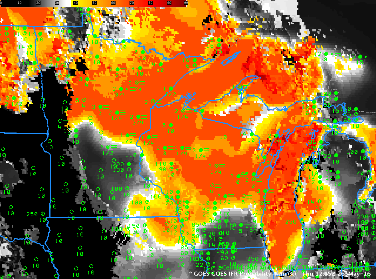
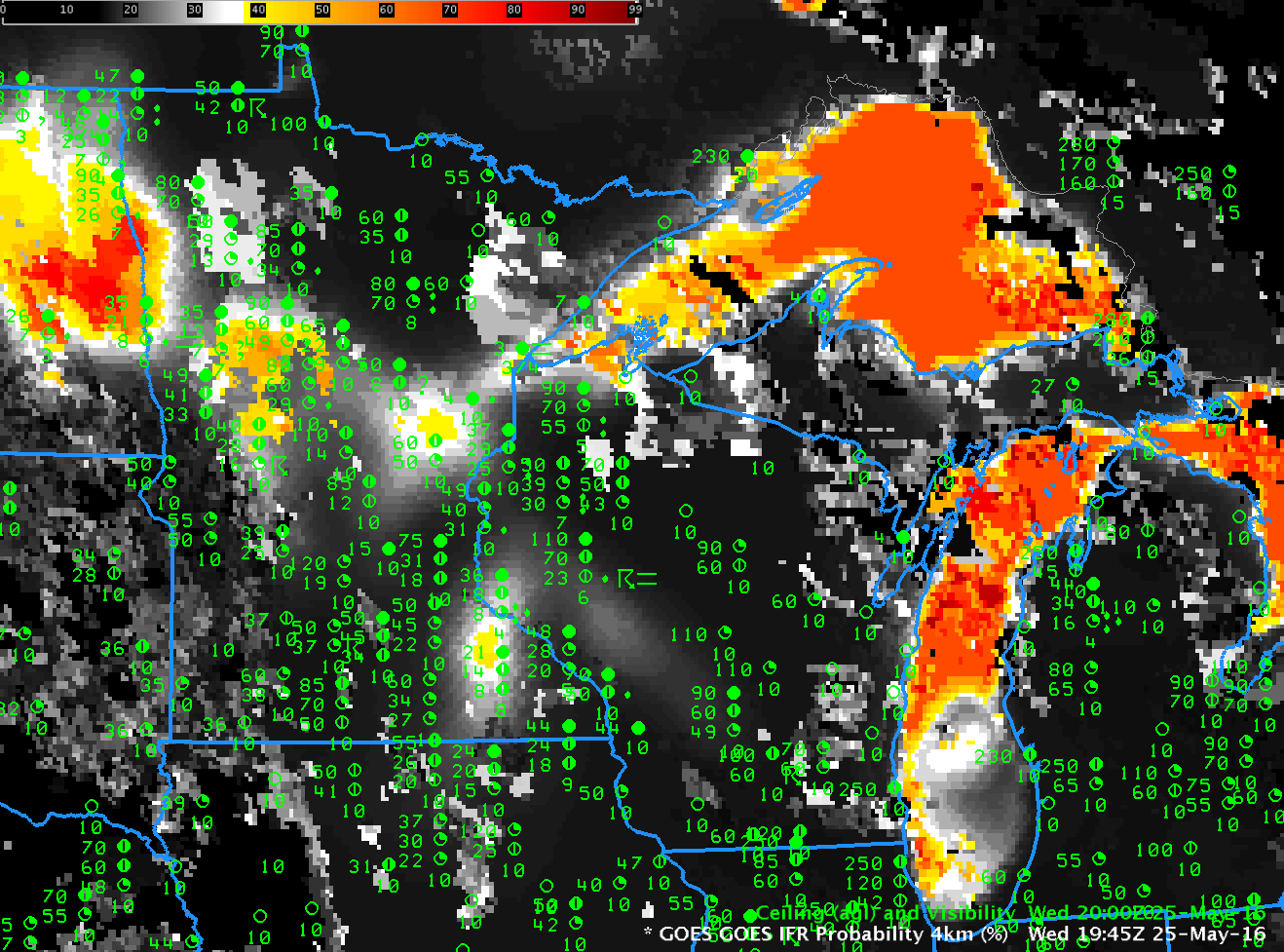
GOES-R IFR Probability fields computed with GOES-13 and Rapid Refresh Data, 1215 UTC on 26 May 2016 along with surface reports of Ceilings and visibilities (Click to enlarge)

High Dewpoint air (upper 50s and low- to mid-60s) has overrun the western Great Lakes, where water temperatures are closer to the mid 40s.  (Water Temperature from Buoy 45007 in southern Lake Michigan).  Advection fog is a result, and that fog can penetrate inland at night, or join up with fog that develops over night.  The image above shows the extent of low visibilities over the upper Midwest and the IFR Probability field early morning on the 26th of May. Lakes Michigan and Superior are diagnosed as socked in with fog. A similar field from 1945 UTC on 25 May similarly shows very high Probabilities over the cold Lakes. Expect high IFR Probabilities to persist over the western Great Lakes until the current weather pattern shifts.

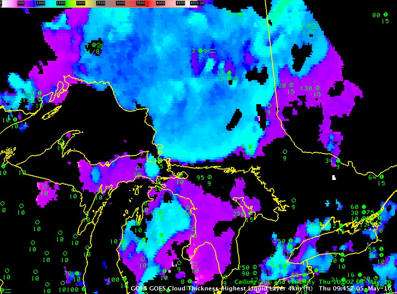
Brightness Temperature Difference Fields can also show stratus over the Great Lakes, of course, but only if multiple cloud layers between the top of the stratus and the satellite do not exist. Convection over the upper Midwest overnight on 25-26 May frequently blocked the satellite’s view of the advection fog. The toggle below, from 0515 UTC on 26 May, shows how model data from the Rapid Refresh is able to supply guidance on IFR probability even in the absence of satellite information about low stratus over the Lakes.

IFRBTD0515_26May2016toggle

GOES-13 Brightness Temperature Difference Fields and GOES-R IFR Probability fields, 0515 UTC on 26 May 2016 (Click to enlarge)

Dense Fog over Southern Iowa

GOESRIFRanim_0315_1215

GOES-R IFR Probability Fields, hourly from 0315 through 1215 UTC on 18 May 2016 (Click to animate)

Dense Fog Advisories were issued by the Des Moines Forecast Office on 18 May as fog developed across southern Iowa. The IFR Probability Field animation, above, articulates where the fog is developing — most of the stations reporting IFR (or near-IFR) conditions are within the region of enhanced IFR Probability, and regions where IFR conditions did not develop show persistent low values of IFR Probability.

Compare the 1015 UTC image of GOES-R IFR Probability and the GOES-13 Brightness Temperature Difference (a traditional way of detecting the presence of low clouds/fog at night), below.  Because the IFR Probability fields incorporate information from the Rapid Refresh Model about low-level saturation, IFR Probability screens out the region in central and northern Iowa where the Brightness Temperature Difference field suggests clouds might be forming (but where surface observations show scant evidence of cloud).

GOES_IFR_BTD_toggle_1015

GOES-R IFR Probability and GOES-13 Brightness Temperature Difference (10.7 µm – 3.9 µm) fields, 1015 UTC on 18 May 2016 (Click to enlarge)

The fog that developed over Iowa was fairly thin and should dissipate quickly under a strong May sun. The GOES-R Cloud Thickness field from 1045 UTC, the last complete field before twilight conditions, below, shows values mostly less than 700 feet with a few pockets of 800-900 feet.  The toggle below shows the GOES-R Cloud Thickness at 1045 UTC and the IFR Probability field 90 minutes later.  Regions with the thickest fog at 1045 UTC do show a persistent signal in the IFR Probability field 90 minutes later.

GOESR_CloudT1045_IFRP_1215toggle

Cloud Thickness and Dissipation Time

CloudThickness_0945_05May2016

GOES-R Cloud Thickness, 0945 UTC on 5 May 2016. Note that Cloud Thickness is not computed in the northeast corner where twilight has begun. This is last scene for northern Ontario and Michigan. (Click to enlarge)

GOES-R Cloud Thickness can be used to make a first guess of when fog and low clouds will dissipate. This is done via a look-up table that is derived from this scatterplot. The y-axis on that plot is the last GOES-R Cloud Thickness field produced before sunrise, such as that shown above, and the x-axis is the number of hours after the plot that clearing is expected, GOES-R Cloud Thickness relates 3.9 µm emissivity to dissipation time based on SODAR observations from off the West Coast, and the scatterplot was derived mostly from observations over the southeast US;  the thickness is that of the lowest water-based cloud field and it’s not computed where multiple cloud layers exist — near Geraldton north of Lake Superior, for example, where IFR Conditions are reported — or near sunrise/sunset.  Values are between 1100 and 1200 feet over northern Lower Michigan,  around 1200 feet over eastern upper Michigan, and around 1200 to as much as 1490 feet over northwest Quebec.  The scatterplot suggests a dissipation time of nearly 4 hours, which would be 1345 UTC.

Imagery below shows low clouds persisting just past 1500 UTC.  For this region where the sun angle is not as high as over the southeast US (where most of the observations used for the scatterplot creation were taken), burn-off took a bit longer.  However, note that GOES-R Cloud Thickness did highlight the thickest clouds that took the longest to dissipate;  so, although the scatterplot underestimated the time of dissipation, Cloud Thickness values did identify which regions would clear last.

A final note: GOES-R Cloud Thickness Dissipation times were computed for Radiation Fog Events, such as the one on 5 May 2016. Dissipation of other fogs that create IFR conditions — Advection Fog, Tule Fog — will not be forecast well with this technique.

GOES13VISLoop_1115_1515_5May2016

GOES-13 Visual (0.63 µm) imagery, 1115-1515 UTC on 5 May 2016 (Click to enlarge)