Monthly Archives: March 2013

Fog/Low Stratus over San Francisco Bay

GOES-R IFR Probabilities computed from GOES-West, hourly from 0800 through 1500 UTC on 29 March 2013

The animation above shows the evolution of fog/low stratus as it moves inland from the Pacific Ocean into San Francisco Bay, and surroundings, on March 29th.  A chief forecast difficulty would be:  Will low ceilings impact San Francisco International Airport?  The TAF issued at 1212 UTC mentioned IFR conditions:

Fog Detection over Snow

GOES-R IFR Probabilities computed from GOES-East (Upper Left), GOES Brightness Temperature Difference (10.7 µm- 3.9 µm ) (Upper Right), Suomi/NPP 1.61 µm Reflectivity (Lower Left), Suomi/NPP Visible Imagery (0.64 µm) (Lower Right)

Snow cover in Spring promotes the development of advection fogs when relatively moist air moves over the snowpack and is cooled to its dewpoint, saturating.  But snowcover is also white when viewed from Satellite, and its presence makes the detection of fog areas difficult.  There are several products that can be used to distinguish between white snow and white clouds, and products that can be used to refine further the difference between stratus decks and fogbanks.

In the imagery above, Suomi/NPP 1-km resolution visible (0.64 µm) data in the bottom right figure show a large region of both clouds and snow over the North Dakota and surrounding US States and Canadian Provinces.  It is very difficult to find the cloud edges that are there.  The 1.61 µm imagery from Suomi/NPP is very helpful in screening out imagery of snow on the ground.  Water clouds are far more effective at reflecting radiation at wavelengths around 1.61 µm than snow or ice (snow and ice both strongly absorb radiation at that wavelength).  Thus, in the bottom left figure, the 1.61 µm reflectivity detected by Suomi/NPP, areas of snow appear dark and areas of water-based clouds are white.  This tells you where water clouds exist, but nothing about how high above the surface those water clouds are.  The brightness temperature difference product from GOES (10.7 µm – 3.9 µm) also highlights in dark regions of water-based clouds, but as with the 1.61 µm reflectivity does not give information about cloud bases.

The GOES-R Fog/Low Stratus IFR Probability neatly distinguished between the stratus deck over western Minnesota (that is not accompanied by IFR conditions at the surface) from the cloudy region over central and northern North Dakota that is accompanied by IFR conditions at the surface, as shown in the plotted observations.  (Thanks to Chad Gravelle for noticing this case today!)

One difficulty in Fog Detection

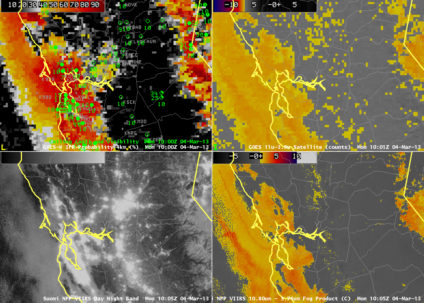
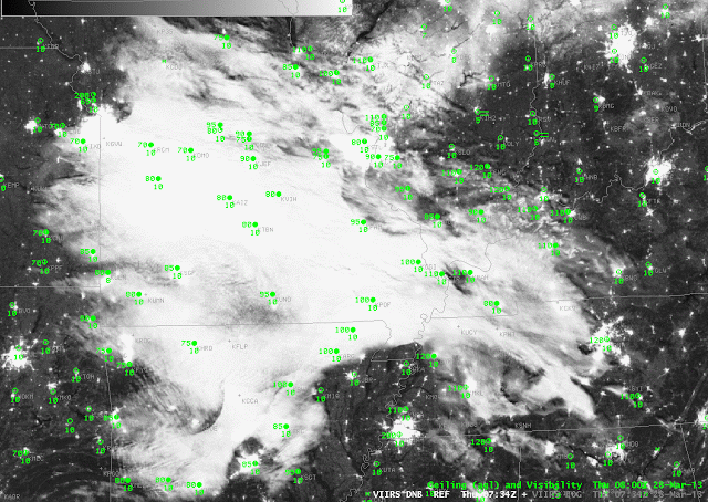
Toggle between Suomi/NPP Day/Night Band (i.e., Night-Time Visible Imagery, 0.70 µm) and Brightness Temperature Difference field (10.8 µm- 3.74 µm) at 0734 UTC on 28 March 2013

The image toggle above shows an area of stratus over central Missouri and surrounding states.  The stratus shows up in both the Night-time visible Day/Night band from Suomi/NPP (March 28th is one day past the Full Moon, so there is plenty of lunar illumination, and indeed lunar shadows from the higher cirrus clouds over Illinois, Kentucky and Tennessee are apparent).  The brightness temperature difference field crisply highlights the region of lower, water-based clouds.  That difference field arises from the differences in emissivity properties of the water-based clouds:  they emit nearly as a blackbody around 11 µm, and not as a blackbody at 3.9 µm.

A key question for this scene is:  is this cloud that is depicted stratus at mid-levels, or is it fog?  From the top (that is, as the satellite views it), a stratus deck will look very much like a fog bank.  The satellite gives little information, however, on how thick the cloud is, or on how close to the ground it sits.  A satellite-only fog detection algorithm, therefore, will include many false positives.

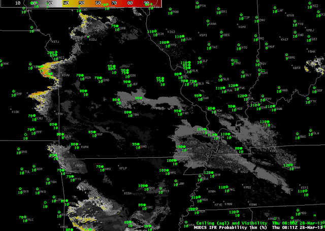
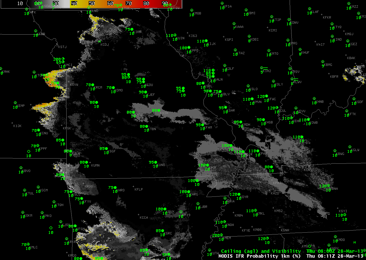
MODIS-based IFR probabilities, 0811 UTC on 28 March 2013

IFR probabilities include data about the surface that are incorporated into the Rapid Refresh Model.   This fused product clarifies where the brightness temperature difference product is detecting mid-level stratus versus low-level fog.  In this case over Missouri, IFR probabilities are very low throughout the scene because saturation at low levels in the Rapid Refresh is not occurring, and therefore IFR probabilities are low.

By blending information about the top of the cloud (the brightness temperature difference product) with information about the bottom of the cloud (the Rapid Refresh model data), a more accurate depiction of the horizontal extent of IFR conditions is achieved.

IFR Probabilities during a Winter Storm

GOES-R IFR Probabilities computed from GOES-East and Rapid Refresh model output, from 0100 through 1400 UTC on March 25 2013

A late winter storm moving through the mid-Altantic states was responsible for an episode of reduced visibilities.  The loop above shows two areas of reduced visibilities initially — one over the Piedmont of Georgia, the Carolinas and Virginia, and one over the Ohio River Valley.  Visibilities decrease as the higher IFR probabilities move in, and, conversely, increase as the higher probabilities move out.  IFR Probabilities over southern Ohio, for example, have a character that suggests the probabilities have been computed chiefly with model data.  Probabilities are somewhat reduced, and the fields are not pixelated (as they are over the Carolina Piedmont, for example).

GOES-R IFR Probabilities computed from GOES-East, Brightness Temperature Difference fields from GOES-East (10.7 µm – 3.9 µm) and from Suomi/NPP (10.8 µm- 3.74 µm) around 0700 UTC on 25 March 2013

The animation of the ~0700 UTC IFR Probability and brightness temperature difference field from both GOES-East and from the polar-orbiting Suomi/NPP, above, shows another strength of the IFR Probability product:  It screens out regions where high stratus give a signal.  The top of a stratus deck and the top of a fog deck may have a very similar brightness temperature difference signal.  By fusing the satellite data with a product that includes surface information (such as output from the Rapid Refresh Model), regions with elevated stratus, which clouds do not significantly impact aviation operations, can be removed from the signal.  Only regions with actual surface observation restrictions are highlighted in the IFR probability signal above.

Cold frontal passage in Oregon

GOES-R IFR Probabilities (Upper Left), GOES-West Brightness Temperature Difference (10.7 µm – 3.9 µm) (Upper Right), Topography (Lower Left), GOES-West Water Vapor Imagery (6.7 µm) (Lower Left), hourly from 0400 through 1700 UTC 20 March 2013.

The animation above of the Fog/Low Stratus and Brightness Temperature difference highlights the difficulty that the traditional brightness temperature difference product encounters when multiple cloud layers are present, as you might expect to be present given the water vapor imagery.  At the beginning of the animation, highest IFR probabilities exist over the elevated terrain that surrounds the Willamette Valley in Oregon.  There were also high probabilities off shore.  As the frontal region moves onshore, IFR probabilities increase on shore.   Note also how the GOES-R IFR Probability field is a more coherent one whereas the traditional brightness temperature difference field from GOES contains many separate areas of return that make it harder to see the big picture.  The brightness temperature difference also suffers from stray light contamination at 1000 UTC — but that contamination does not propagate into the GOES-R IFR probability field.

GOES-R IFR Probabilities computed from GOES-West (Upper Left), GOES-West Brightness Temperature Difference (10.7 µm – 3.9 µm) (Upper Right), Topography (Lower Left), Toggle between Suomi/NPP Brightness Temperature Difference (10.8 µm – 3.74 µm) and Day/Night Band, all imagery near 1000 UTC on 20 March 2013

The imagery above shows how straylight contamination in the shortwave IR (3.9 µm) can influence the brightness temperature difference.  The GOES imagery shows the effects (just at this 1000 UTC image, which is also included in the animation above), but that ‘contamination’ does not propagate strongly into the GOES-R IFR Probability.  Note also that the Suomi/NPP Brightness Temperature Difference shows none of the stray light contamination.  Lunar illumination  allows the nighttime visualization of the clouds off the west coast of the US.  As this frontal band moves over Oregon, reduced visibilities result, but only the GOES-R IFR probabilities accurately capture the location of the frontal band because of the multiple cloud layers that exist.

GOES-produced IFR Probabilities over Alaska

GOES-R IFR Probabilities from GOES-West over Alaska and the Bering Sea, half-hourly from 0000 UTC through 1500 UTC on 18 March 2013

Even though Alaska is at high latitudes, and GOES Imagery there is burdened with degraded resolution, the temporal aspect of the data can give useful information.  As an example, consider the animation of GOES-R IFR probabilities near Bethel Alaska along the west coast of Alaska.  Note that Bethel AK, in the center (nearly) of the image, is reporting MVFR/VFR conditions, with IFR conditions along the coast — at Kipnuk and Toksook — and offshore at Mekoryuk on Nunivak Island as well as St. George and St. Paul Islands.  The fused GOES/Rapid Refresh data is able to delineate correctly the regions with IFR conditions along the coast and offshore from the regions with MVFR/VFR conditions to the east.

GOES-R IFR Probabilities computed from MODIS data over western Alaska, 0826 UTC 18 March 2013

MODIS data can also give information over Alaska, and the 1-km resolution offers important information.  Bethel sits in the region of relatively low IFR probabilities west of the higher probabilities along the coast.

Coastal Stratus over southern California

Hourly imagery of GOES-R IFR Probability computed from GOES-West, from 0200 UTC through 1400 UTC 14 March 2013

Hourly imagery of GOES-R IFR Probability from the overnight/early morning of 14 March 2013 shows the typical advance inland of stratus along coastal southern California.  Several aspects of this loop bear mention.  In the 0200 UTC, the division between daytime predictors (to the left) and nighttime predictors (to the right) is evident extending mostly north-south over the Ocean.  Visibilities at Los Angeles International Airport (LAX) drop to IFR conditions as the diagnosed IFR probabilities push inland.  Note also the good relationship between high probabilities and low visibilities along the coast north of San Diego.

There is a push inland of higher probabilities at 1000 UTC in the loop above that is not well reflected in the observations.  This occurs because of stray light contamination in the brightness temperature difference channel that is obvious in the animation below.  Note also how the many ‘false positives’ in the brightness temperature difference product over land in Southern California, differences that are attributable to emissivity differences in the surface, not to the presence of liquid water clouds, are effectively screened out in the GOES-R IFR Probability product.

Traditional Brightness Temperature Difference product (10.7 µm – 3.9 µm) from GOES-West (mostly).  Note that the ‘seam’ between GOES-East data and GOES-West data is present in the eastern part of the imagery.  Hourly data from 0200 through 1400 UTC on 14 March 2013.

Resolution Issues over the Pacific Northwest

GOES-R IFR Probabilities computed from GOES-West (Upper Left), GOES-E/W Brightness Temperature Difference (10.7 µm – 3.9µm) (Upper Right), GOES-R Cloud Thickness (Lower Left), Suomi/NPP VIIRS Brightness Temperature Difference  (Lower Right)
As on top, but with MODIS Brightness Temperature Difference (11 µm – 3.7 µm) in the bottom right.

The imagery above underscores the power of higher resolution on fog detection.  The images on the right side of the images are brightness temperature difference fields, the heritage method for detecting fog and low stratus.  The GOES field (top right) actually includes data from GOES-East (eastern Washington and points east — a faint seam is discernible in the image) and GOES-West (western Washington).  Pixel size over Washington is large — 6 or 8 kilometers (vs. 4 kilometers at the subsatellite point).  In contrast, Suomi/NPP VIIRS data and MODIS data (bottom right) has a resolution of 1 km.  The brightness temperature difference from MODIS and VIIRS more easily resolves the fine-scale structure of the topographically influenced or topographically constrained fog and low stratus.  The brightness temperature difference field from GOES is one of the predictors used to generate the IFR Probabilities shown in the upper right.  When poor resolution smears out the horizontal domain of the fog and low stratus in the brightness temperature difference field, you might expect a similar effect on the IFR probabilities.

As above, but with MODIS-based GOES-R IFR Probabilities in the lower right

 MODIS data can be used to compute IFR probabilities.  Compare the lower right and upper left figures.  High MODIS IFR Probabilities are far more restricted to regions where IFR conditions are observed.  In contrast, GOES-based IFR probabilities seem to leak into regions where IFR conditions are not reported.

The higher resolution MODIS-based IFR Probabilities (and coming soon, Suomi/NPP-based IFR probabilities) nicely complement the higher temporal resolution of the GOES imagery.  Ideally, use of the changes in the GOES-based IFR probabilities shows how IFR conditions evolve over the course of a night.  These changes should be tempered with knowledge of the limitations of the horizontal resolution of GOES that are highlighted in the above imagery.

Fog near San Francisco

GOES-R IFR Probabilities computed from GOES-West (Upper Left), GOES-West Brightness Temperature Difference (10.7 µm – 3.9 µm) (Upper Right), Suomi/NPP VIIRS Day/Night Band (Lower Left), Suomi/NPP VIIRS Brightness Temperature Difference (10.8 µm- 3.74 µm) (Lower Right), all images near 1000 UTC on March 4 2013.

A high-impact fog event on March 1st led to a Group Stop at SFO International.  The synoptic conditions that supported fog development on 1 March (Images from 1 March are shown at the bottom of this blog post) persisted through the weekend along the West Coast, and fog was again observed on Monday morning, 4 March and the four images above show results from fog detection schemes for that date.  The GOES-R Fog/Low Stratus IFR Probability field shows that the highest probability of IFR conditions is occurring where IFR and near-IFR conditions are observed.  Note the benefits of the high-resolution Suomi/NPP VIIRS data.  Sharp edges to the low cloud field are ably captured in central Santa Clara County.  There are also benefits to using the near infrared and infrared channels to detect regions of low clouds in urban areas, where bright lights can dazzle the Day/Night band so that small breaks in the clouds, as detected just south and west of southern San Francisco Bay, cannot be discerned in the visible.  Compare the differences in the 1-km data from VIIRS to the nominal 4-km resolution of present GOES in the imagery above.  Note also that the brightness temperature difference helps distinguish between snow and clouds over the Sierra Nevada.

GOES-R IFR Probabilities computed from GOES-West, hourly, from 0400 UTC to 1600 UTC on 4 March 2013

The animation, above, of GOES-R IFR Probabilities helps describe and define the region of evolving IFR conditions early on March 4th.

Figures provided by Warren Blier, WFO MTR.

Warren Blier from NWS in MTR sent along an email about the event on March 1st.  The screen capture above shows MODIS-based GOES-R IFR probabilities (on the right) compared with the GOES-West ‘traditional’ unenhanced  brightness temperature difference.  The higher spatial resolution of MODIS and of VIIRS really does pick up the details.  The image below is the 1000 UTC image created using GOES-West data, and the comparison between the MODIS image above and the GOES image below shows the power of MODIS resolution.

GOES-R IFR Probabilities computed using GOES-West data, 1000 UTC on 1 March 2013

An animation of GOES-R IFR probabilities from 0000 through 1600 UTC on 1 March shows the highest IFR probabilities increasing near SFO after 0900/1000 UTC on the first.

Hourly imagery of IFR probabilities computed from GOES-West, 0000 through 1600 UTC on March 1st