Category Archives: Suomi/NPP

Fog after convection in Virginia and North Carolina

GOES-R IFR Probability fields, hourly from 0215 UTC through 1115 UTC on 28 September 2016 (Click to enlarge)

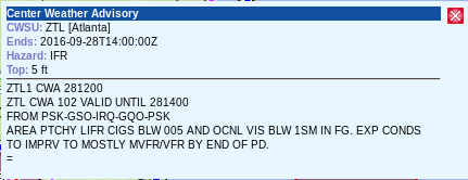
IFR and Low IFR Conditions developed over parts of Virginia and the Carolinas Piedmont Region during the morning of 28 September 2016. The screengrab below, from the Aviation Weather Center, shows the areal extent of the reduced visibilities and/or low ceilings. (The text of the IFR Sigmet is here.) Fog over southeastern Virginia is developing under multiple cloud decks associated with the convection near a front. IFR Probabiities in this region are determined by Rapid Refresh data that shows low-level saturation; the flat-looking field over that region is characteristic of model-only IFR Probability fields. Farther to the southwest, over western North Carolina, IFR Probabilities are determined by both satellite and model data; notice how pixelated the data are in that region.

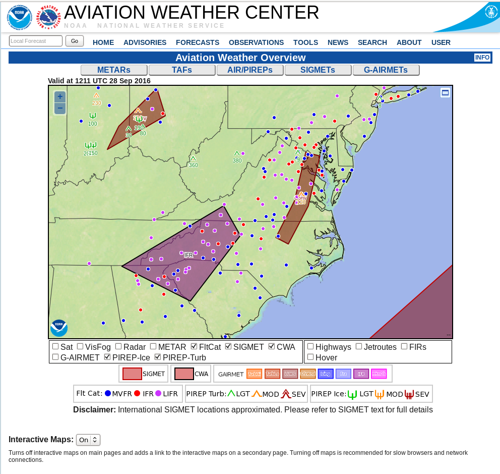
Screengrab from the Aviation Weather Center at 1215 UTC on 28 September 2016 (Click to enlarge)

Suomi NPP overflew the eastern United States shortly after 0730 UTC, and the toggle below shows the Day Night Visible Band and the Brightness Temperature Difference field (11.45 – 3.74 ). Water-based clouds (yellow and orange in the enhancement used) are detected just to the west of cirrus and mixed-phase clouds (black in the enhancement used). The 0737 UTC IFR Probability field, at bottom, had model-data only as predictors in regions where Suomi NPP shows multiple cloud layers. Note also that the 1-km resolution of Suomi NPP is resolving the developing valley fogs in the Appalachian mountains of Ohio, West Virginia and Kentucky. There are only a few pixels in the IFR Probability field that are suggesting valley fog development — but note in the end of the animation at the top of this post that more valley pixels show IFR Probability signals. When GOES-R is flying, its superior (to GOES-13) 2-km resolution should mitigate this too-slow identification of valley fogs.

Suomi NPP Day Night Band Visible (0.70) and Brightness Temperature Difference (11.45 – 3.74) fields at 0736 UTC on 28 September 2016 (Click to enlarge)

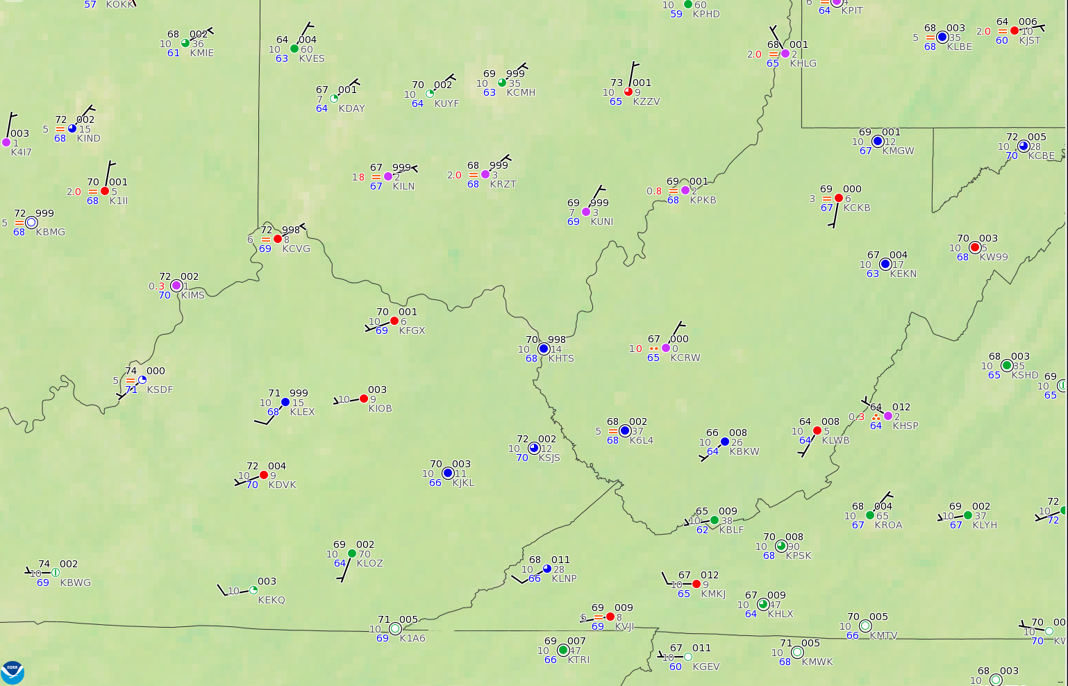
GOES-R IFR Probability fields at 0737 UTC, and surface observations of ceilings and visibilities at 0800 UTC (Click to enlarge)

Low Ceilings and reduced visibilities over the Ohio Valley

Surface Observations at 1200 UTC on 24 June 2016 (Click to enlarge)

A screen capture from this site at 1215 UTC on 24 June 2016, above, shows IFR Conditions (Red) and Low IFR Conditions (Purple) over the upper Ohio River Valley and surrounding states. The IFR Probability field for the same time, below, shows high probabilities in roughly the same regions that have IFR or Low IFR conditions. The Brightness Temperature Difference field, also displayed in the toggle below, gives little information at this time of day. A benefit of the GOES-R IFR Probability field is that it contains a coherent signal through sunrise.

GOES-R IFR Probability fields and GOES-13 Brightness Temperature Difference Fields (3.9 µm – 10.7 µm) at 1215 UTC on 24 June 2016 (Click to enlarge)

The toggle at 0915 UTC, below, before sunrise, shows a second benefit of IFR Probability fields: a useful signal in regions with cirrus clouds. High clouds, of course, prevent GOES-13 from viewing the development of fog/low stratus near the surface. The Rapid Refresh model data on low-level saturation that are part of the IFR Probability Field computations give quality information in regions of cirrus. In the example below, developing IFR conditions are depicted (the yellow enhancement that shows IFR Probabilities around 40%) over much of northern Kentucky and southern Ohio. This is under a region of cirrus (black in the enhancement used for the brightness temperature difference) north of a convective system that sits over southeastern Kentucky and eastern Tennessee.

GOES-R IFR Probability fields and GOES-13 Brightness Temperature Difference Fields (3.9 µm – 10.7 µm) at 0915 UTC on 24 June 2016 (Click to enlarge)

The waning full moon provided ample illumination for the Suomi NPP Day/Night Band Imagery, shown below, from 0736 UTC on 24 June 2016. The cirrus shield, mid-level clouds and developing valley fogs are all apparent.

Suomi NPP Day/Night band imagery, 0736 UTC on 24 June 2016 (Click to enlarge)

Fog over the Tennessee River Valley

GOES-R IFR Probability fields, every two hours from 0115 through 1315 UTC on 17 February 2016 (Click to enlarge)

GOES-R IFR Probability fields showed large values over parts of Kentucky and Tennessee during the overnight hours on 16-17 February 2016, as shown in the animation above (every 2 hours from 0115 through 1315 UTC). (IFR or near-IFR Conditions were present over the region of enhanced IFR Probabilities) For much of the overnight hours, mid-level and high clouds prevented an unobstructed satellite view of low clouds, so Rapid Refresh model output was the principle driver in IFR Probabilities. When that happens, the character of the IFR Probability field is less pixelated (it’s a flatter field) and values are smaller. At the end of the animation — 1315 UTC — satellite observations of low clouds have improved and the GOES-R IFR Probability field is (1) more pixelated, as expected when satellite data are used and (2) showing higher values because Satellite Predictors can be used in the computation of IFR Probability.

MODIS data from Terra and Aqua satellites can also be used to compute IFR Probability fields, and the high spatial resolution of the MODIS instrument (1-km vs. nominal 4-km on GOES) can yield superior results for valley fogs, for example (The effects of some rivers are apparent in the 0354 UTC image over western Tennessee, for example). For a large-scale event as above, however, GOES-based resolutions can be adequate. The toggle of MODIS-based GOES-R IFR Probabilities at 0354 UTC and 0810 UTC is shown below. Patchy clouds (that prevent MODIS from viewing low clouds) are more apparent in the 0354 UTC image than in the 0810 UTC image.

MODIS-based GOES-R IFR Probabilities, 0354 and 0810 UTC on 17 February 2016 (Click to enlarge)

Suomi NPP Overflew the Tennessee River valley just after midnight local time, and the toggle of the Day Night band and the Brightness Temperature Difference field (11.45 – 3.74) is shown below. Extensive cloud cover is apparent. The importance of the IFR Probability fields is that it incorporates surface information (from the Rapid Refresh predictions of saturation in the lowest 1000 feet of the model atmosphere) so that fog and low stratus that impacts transportation by reducing visibilities can be distinguished from mid-level stratus that has a smaller impact.

Suomi NPP Brightness Temperature Difference fields (10.8 µm – 3.74 µm) and Day Night band visible imagery (0.70 µm) at 0735 UTC on 17 Feburary 2016 (Click to enlarge)

Small-scale Fog Event near Puget Sound

GOES-R IFR Probabilities computed with GOES-15 and Rapid Refresh Data, 1100-2200 UTC on 9 February 2016 (Click to enlarge)

GOES-R IFR probabilities on Tuesday 9 February captured the development of a small-scale fog event in/around the southern part of Puget Sound in Washington State. The animation above shows high IFR Probabilities developing shortly before sunrise and persisting through most of the day in a region including Shelton, Olympia, Tacoma and Seattle.

MODIS visible data, below, from the Terra Satellite overpass shortly after 1800 UTC, below, shows the fogbank over the most of Puget Sound, extending inland only over the southern part of the sound.

MODIS Visible Imagery (0.65 µm), 1822 UTC on 9 February (Click to enlarge)

Suomi NPP viewed Puget Sound on two consecutive overpasses on 9 February, and visible imagery from those passes, just before 2000 UTC and near 2130 UTC, are shown below. Fog Dissipation is apparent in the later image, which is consistent with the animation of IFR Probability at the top of this post, which animation shows IFR Probabilities declining in value after 2100 UTC.

Suomi NPP Visible Imagery (0.64 µm), 1953 and 2122 UTC on 9 February (Click to enlarge)

Fog vs. Stratus over the Pacific Northwest

Brightness Temperature Difference (10.7 µm – 3.9 µm) from GOES highlight regions of water-based clouds: water-based clouds emit 10.7 µm radiation nearly as a blackbody does, but those clouds do not emit 3.9 µm radiation as a blackbody. Thus, the brightness temperature computed from the radiation detected by the satellite (GOES-15 in this case) — a computation that assumes a blackbody emission — is relatively cooler for the 3.9 µm data compared to the 10.7 µm data. A water-based cloud is normally stratus, and the pertinent question for aviation purposes (for example) is: Is the ceiling of that cloud near the surface? (That is: Is the stratus also a fog bank, or is it “just” mid-level stratus?)

GOESIFRP_BTD_15December2015_0500UTCtoggle

GOES-15 Brightness Temperature Difference (10.7 µm – 3.9 µm) and GOES-based GOES-R IFR Probabilities, 0500 UTC 15 December 2015 (Click to enlarge)

The toggles above (0500 UTC) and below (0900 UTC) show how the GOES-R IFR Probability fields capably screen out many regions of mid-level stratus. This is achieved by fusing the brightness temperature difference information with data from the Rapid Refresh Model. If the lowest 1000 feet of the Rapid Refresh Model is not near saturation, probabilities of IFR conditions are reduced.

GOESIFRP_BTD_15December2015_0900UTCtoggle

As above, but at 0900 UTC 15 December 2015 (click to enlarge)

GOESIFRP_BTD_15December2015_1200UTCtoggle

As above, but at 1200 UTC 15 December 2015 (click to enlarge)

Toggles from 1200 UTC (above) and 1400 UTC (below) continue to show IFR Conditions mostly confined to regions near the Willamette Valley in eastern Oregon — banked up against the higher terrain to the east of the Willamette, and also over the higher terrain of northeastern Oregon (Click here for a toggle between the 1400 UTC IFR Probability field and Topography). IFR Conditions are a function of ceilings above ground (not above Mean Sea Level), so it’s important to recognize the influence of topographic features on an IFR Probability field. Fog/Low stratus can bank up against a topographic feature, and/or it can shroud the top of a topographic feature.

Note also how at 1400 UTC high clouds have impinged upon extreme northwest Oregon and coastal western Washington. In these regions IFR conditions nevertheless persist under the high clouds, but satellite data alone does not indicate low cloudiness. In this region, the inclusion of Rapid Refresh data in the GOES-R IFR Probability algorithm allows the IFR Probability field to continue to provide useful information about the presence of fog/low stratus.

GOESIFRP_BTD_15December2015_1400UTCtoggle

As above, but at 1400 UTC 15 December 2015 (click to enlarge)

MODIS and Suomi NPP afforded high-resolution images of the fog/stratus banks over the Pacific Northwest on 15 December. The brightness temperature difference fields and MODIS-based IFR Probability fields from MODIS at 0533 and 0945 UTC, below, support the observations from the coarser-resolution GOES fields above.

MODISIFRP_BTD_15December2015_0533UTCtoggle

As above, but for MODIS data at 0533 UTC 15 December 2015 (click to enlarge)

MODISIFRP_BTD_15December2015_0945UTCtoggle

As above, but for MODIS data at 0945 UTC 15 December 2015 (click to enlarge)

GOES-R IFR Probability fields are not yet computed using data from the Suomi NPP Satellite, but the Day Night band and the Brightness Temperature Difference field give information about the presence of cloudiness. For the case of Suomi NPP data, however, it’s more important to consider surface-based observations to confirm regions of low clouds/fog or mid-level stratus. Note also that December 15 was shortly after a New Moon, and the crescent moon that could give illumination was below the horizon (that is, it had set) at 0918 and 1059 UTC.

Note that Suomi NPP Near-Constant Contrast Day Night Band imagery was scheduled to start flowing in to AWIPS II on 14 December 2015 via the SBN. It should be available in NWS offices now.

SNPPBTD_DNB_15December2015_0918UTCtoggle

Suomi NPP Day Night Band Visible Imagery (0.70 µm) and Brightness Temperature Difference (10.35 µm – 3.74 µm), 0918 UTC 15 December 2015 (Click to enlarge)

SNPPBTD_DNB_15December2015_1059UTCtoggle

Suomi NPP Day Night Band Visible Imagery (0.70 µm) and Brightness Temperature Difference (10.35 µm – 3.74 µm), 1059 UTC 15 December 2015 (Click to enlarge)

Are IFR Conditions Present?

Suomi NPP Visible (0.70 µm) Day Night Band Imagery and Infrared Brightness Temperature Differences (11.45 µm – 3.74 µm), 0731 UTC on 24 November 2015 (Click to enlarge)

Low clouds (with a sharp southern edge) were over northern Wisconsin during the early morning of 24 November 2015. Are IFR Conditions present? Can you tell from the satellite imagery alone? The cloud bank stretched over northern Wisconsin seems thick compared to the bank of clouds over northeastern Wisconsin (centered on southern Green Bay). The city lights of Duluth are not visible in the same way that the city lights of Green Bay are in the Day Night band imagery. Clouds in general are distinct with the near-full moon providing ample illumination.

Both GOES and MODIS Brightness Temperature Difference fields, below, show a signal consistent with low clouds over most of northern WI and adjacent regions. But are there IFR Conditions?

GOES-13 Brightness Temperature Difference (10.7 µm – 3.9 µm) Fields (0730 UTC) and MODIS Brightness Difference Fields (11 µm – 3.9 µm) (0749 UTC)

IFR Probability fields blend the information available from satellite (are water-based clouds present?) with model output to yield a refined diagnostic of IFR Conditions. If there is saturation in the lowest levels (the lowest 1000 feet) of the model, then Probabilities of IFR Conditions are increased. If the lowest levels of the model are relatively dry, in contrast, then IFR Probabilities are reduced. On the morning of 24 November, the latter condition occurred over northern Wisconsin. IFR Probabilities computed from MODIS and GOES-13 satellite values are shown below. Probabilities are very low over most of Wisconsin where mid-level stratus (with varying bases) was present: IFR conditions were not generally observed in the regions where water-based clouds were indicated by the satellite. Mid-level stratus can look, from the top, very similar to fog, but it’s impossible for the satellite alone to discern what’s happening at the cloud base. Model data helps the IFR Probability algorithm screen out regions where mid-level stratus is occurring.

MODIS-based GOES-R IFR Probabilities (0751 UTC), GOES-13-based GOES-R IFR Probabilities (0731 UTC), and GOES-based GOES-R IFR Probabilities with surface observations of ceilings and visibilities (Click to enlarge)

Using MODIS and GOES IFR Probabilities to gauge fog motion in the Pacific Northwest

MODIS-based brightness temperature difference fields, ~0550 and ~1000 UTC on 6 July (Click to enlarge)

MODIS-based Brightness Temperature Difference fields, above, from 0547 (Terra) and 0958 (Aqua) detect a large area of marine stratus over the Pacific Ocean that is penetrating inland up river valleys along the coasts of Washington and Oregon. Dark reatures that are consistent with higher clouds are also present over southern Oregon. GOES-R IFR Probability fields can be computed from MODIS data, and those fields (below) show high probabilities along the coast, in regions where IFR or near-IFR conditions are observed. Aspects of the GOES-R IFR Probability field deserve comment. Where high clouds are present in the MODIS data, GOES-R IFR Probabilities are largely controlled by model-based fields that are typically smooth. This is the case over the northwest corner of the IFR Probability field, for example, and also off the southern Oregon coast at ~0550 UTC. The blocky nature of the IFR Probability fields off the central Oregon coast at ~0550 UTC is likely related to model relative humidity fields that show saturation both near the surface and aloft.

MODIS-based GOES-R IFR Probabilities, ~0550 and ~1000 UTC on 6 July 2015 (Click to enlarge)

Suomi NPP Day Night Band visible imagery had ample illumination early on 6 July with a waning gibbous moon. Imagery below from 1000 UTC (very close to the Aqua pass) also shows thin tendrils of fog moving up river valleys. The VIIRS instrument that provides the Day Night imagery is only on one satellite, however, (compared to MODIS on both Aqua and Terra) so such views are infrequent.

Suomi NPP Day Night Band Visible imagery and Brightness Temperature Difference fields at 0959 UTC, 6 July 2015 (Click to enlarge)

MODIS and Suomi NPP imagery suggest fog is penetrating preferentially into river valleys along the west coast. This should color the interpretation of GOES-based GOES-R IFR Probabilities. GOES-15 lacks the horizontal resolution to resolve fully most river valleys (Rapid Refresh data, similarly, does not resolve small valleys); however, GOES-15 does have excellent temporal resolution, and combining that with the intermittent information from polar orbiters such as Terra, Aqua and Suomi-NPP provides a fuller picture of the evolution of near-surface IFR conditions. The animation of GOES-R IFR Probabilities from GOES-15 is shown below.

GOES-15 based GOES-R IFR Probabilities, 0445-1345 UTC, 6 July 2015 (Click to enlarge)

Dense Fog over Iowa and Illinois

Front page of the National Weather Service in the Quad Cities, Monday morning 29 June 2015 (Click to enlarge)

Dense fog developed over the mid-Mississippi Valley early on Monday, 29 June 2015, and Dense Fog Advisories were hoisted by the DVN WFO, as shown above. How did the GOES-IFR Probabilities (and other products) capture this event? The animation below shows the evolution of surface visibilities at 0600, 0800 and 1000 UTC. IFR Conditions have developed by 0600 UTC and they subsequently expand.

Surface Visibilities (Statute Miles) over Iowa, 0600, 0800 and 1000 UTC, 29 June 2015. IFR Conditions are highlighted in white (Click to enlarge)

The Day Night band suggests clouds are present over parts of Iowa at 0707 UTC, but the waxing gibbous moon has set by 0848 UTC (below), and the lack of reflected moonlight at the later time precludes cloud detection. The brightness temperature difference (11.45µm – 3.74µm) from Suomi NPP can detect the tops water-based low clouds and it does confirm that the clouds have not vanished at 0848 UTC despite the lack of signal in the Day Night band. The brightness temperature difference field includes signals (black in the enhancement used) that suggest the presence of cirrus clouds.

VIIRS_DNB__REF_20150629_toggle_0707_0848

Visible Imagery from the Suomi NPP Day Night Band, 0707 and 0848 UTC on 29 June 2015 (Click to enlarge)

Suomi NPP Brightness Temperature Difference (11.45µm – 3.74µm) at 0707 UTC and 0848 UTC (Click to enlarge)

MODIS data can be used to compute IFR Probability fields. These fields are not available frequently, although they do present a high-resolution view of events when available. Two overpasses, at 0408 (Terra) and 0817 (Aqua), provided imagery early on 29 June. The MODIS data suggests the development of a large area of fog. What does GOES data show? Click here for a comparison of MODIS and GOES at 0408 UTC, and here for a comparison of MODIS and GOES at 0817 UTC). The chief difference between MODIS and GOES is somewhat higher values at the earlier time, and sharper edges (as might be expected given the resolution differences) at both times.

MODIS-based GOES-IFR Probabilities, 0408 and 0817 UTC on 29 June 2015 (Click to enlarge)

GOES-R IFR Probabilities computed from GOES-13 have a temporal resolution that allows for monitoring of fog development, and values increase rapidly after 0500 UTC over eastern Iowa, in accord with the development of IFR observations shown above. Brightness Temperature Difference fields (bottom) also suggest the development of low clouds over Iowa. However, there are places where high clouds prevent a signal and the rising sun (and its 3.9 µm radiation) mean the signal is reduced at the end of the animation. GOES-R IFR Probabilities maintain a coherent signal through sunrise.

GOES-based GOES-R IFR Probabilities, 0400-1215 UTC on 29 June 2015 (Click to enlarge)

GOES-13 Brightness Temperature Difference (10.7 µm – 3.9 µm), 0400-1215 UTC, 29 June 2015 (Click to enlarge)

Resolution Matters

GOES-R IFR Probabilities computed from MODIS data and from GOES-15 data, ~1000 UTC on 22 June 2015 (Click to enlarge)

GOES-R IFR Probability was created with an eye towards using data from GOES-R (currently scheduled for launch at the end of March 2016). GOES-R will have better spatial, temporal and spectral resolution than the present GOES. A benefit of better spatial resolution is shown in the toggle above between present GOES (nominal 4-km resolution — vs. the nominal 2-km resolution that will be on GOES-R) and MODIS (1-km resolution). The small valleys along the northern California coastline are far better resolved. The fog/low clouds over San Francisco bay is also better resolved (and the same could be said for the Salinas Valley, south of Monterey Bay if this scene were shifted slightly south). (You might notice a slight 1-pixel shift between MODIS and GOES-15 IFR Probabilities. GOES-15 navigation is compromised by the lack of star-tracking data, so MODIS data are probably better navigated.)

GOES-15 Brightness Temperature Difference (10.7 µm – 3.9 µm) and GOES-R IFR Probabilities, 1000 UTC on 22 June 2015 (Click to enlarge)

IFR Probabilities are derived from GOES-15 brightness temperature difference fields, and a benefit of the IFR Probabilities is obvious above. Brightness Temperature Differences can be driven by emissivity differences in soil. These false positives over Nevada (from the point of view of fog detection) are easily removed if the Model Data does not show low-level saturation.

Suomi NPP Day/Night band imagery, Brightness Temperature Difference Fields (11.45 µm – 3.74 µm), and 3.74 µm Image, 0921 UTC on 22 June 2015 (Click to enlarge)

Suomi/NPP’s early morning overpass also detected the presence of fog/low stratus over the valleys along the northern California coast. The Brightness Temperature Difference field shows things distinctly. The Day-Night Visible imagery shows little in the way of fog on this day, as the waxing crescent moon had already set so no lunar illumination was present. The Day Night band is included here because it shows a very bright wildfire south of Lake Tahoe. That feature is also present in the 3.74 µm imagery. Fog and stratus is also evident in the 3.74 µm imagery, detectable based on its very smooth appearance.

Fog over Coastal California

GOES-R IFR Probabilities computed from GOES-West and Rapid Refresh Data, 0300-1200 UTC on 29 May 2015 (Click to enlarge)

GOES-R IFR Probability fields are challenged most days by the diurnal penetration of coastal fog and stratus that occurs overnight along the California Coast. In the animation above, IFR Probabilities increase in regions along the coast, and also in valleys (such as the Salinas Valley) where fog moves inland. Note above how Monterey, Watsonville and Paso Robles all show IFR (or near-IFR) conditions as the IFR Probabilities increase. The same is true farther north at Santa Rosa and at Marin County Airport, and farther south at Avalon, Ontario, Point Mugu and LA International. IFR Probability fields routinely do capture these common fog events.

The Brightness Temperature Difference Field (10.7 µm – 3.9 µm), below, captures the motion of these low clouds as well. However, numerous ‘false positive’ signals occur over the central Valley of California (likely due to differences in soil emmissivities). The GOES-R IFR Probability field can screen these regions out because the Rapid Refresh data in the region does not show saturation in the lowest kilometer. Note also how the Brightness Temperature Difference field gives little information about low clouds where high clouds are present (over the Pacific Ocean in the images below). IFR Probability fields, however, do maintain a strong signal there because data from the Rapid Refresh strongly suggests the presence of low clouds/fog.

GOES Brightness Temperature Difference Fields, 0400-1200 UTC on 29 May 2015 (Click to enlarge)

Suomi NPP makes an overflight over the West Coast each day around 1000 UTC, and the toggle of the Day Night Band and the Brightness Temperature Difference field (11.45 µm – 3.74 µm) is shown below. The moon at this time was below the horizon, so illumination of any fog is scant; the brightness temperature difference field does highlight regions of water-based clouds (that is, stratus); however, it does not contain information about the cloud base. In other words, it’s difficult to use the brightness temperature difference product alone to predict surface conditions.

1010 UTC Imagery from Suomi NPP VIIRS Instrument: Day Night Visible Band (0.70µm) and Brightness Temperature Difference Field (11.45µm – 3.74µm) (Click to enlarge)

GOES-14 is in SRSO-R mode, and its view today includes the west coast. The animation below shows the erosion of the fog after sunrise at 1-minute intervals. (Click here for mp4, or view it on YouTube). (Click here for an animation centered on San Francisco).

GOES-14 Visible (0.6263 µm) animation, 29 May 2015 [click to play very very large animation]

GOES-R Fog Product Examples

Fog detection fusing GOES, Terra/Aqua or Suomi/NPP Satellite data with Model output