Monthly Archives: September 2013

IFR Conditions on the West Coast as a front passes

GOES_IFR_PROB_20130930_loop

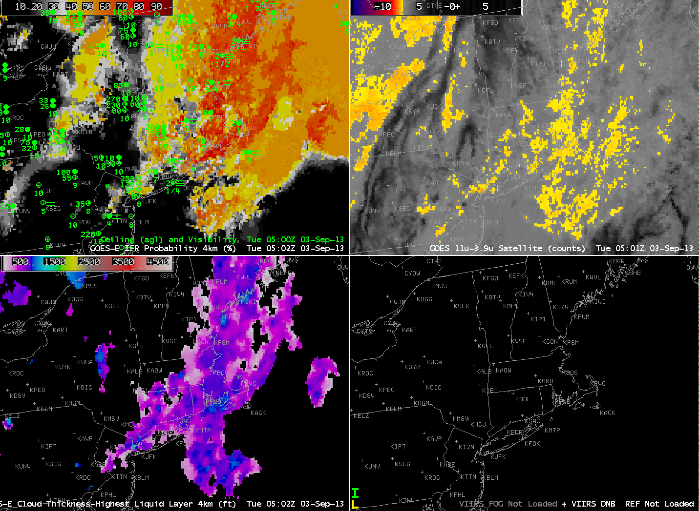
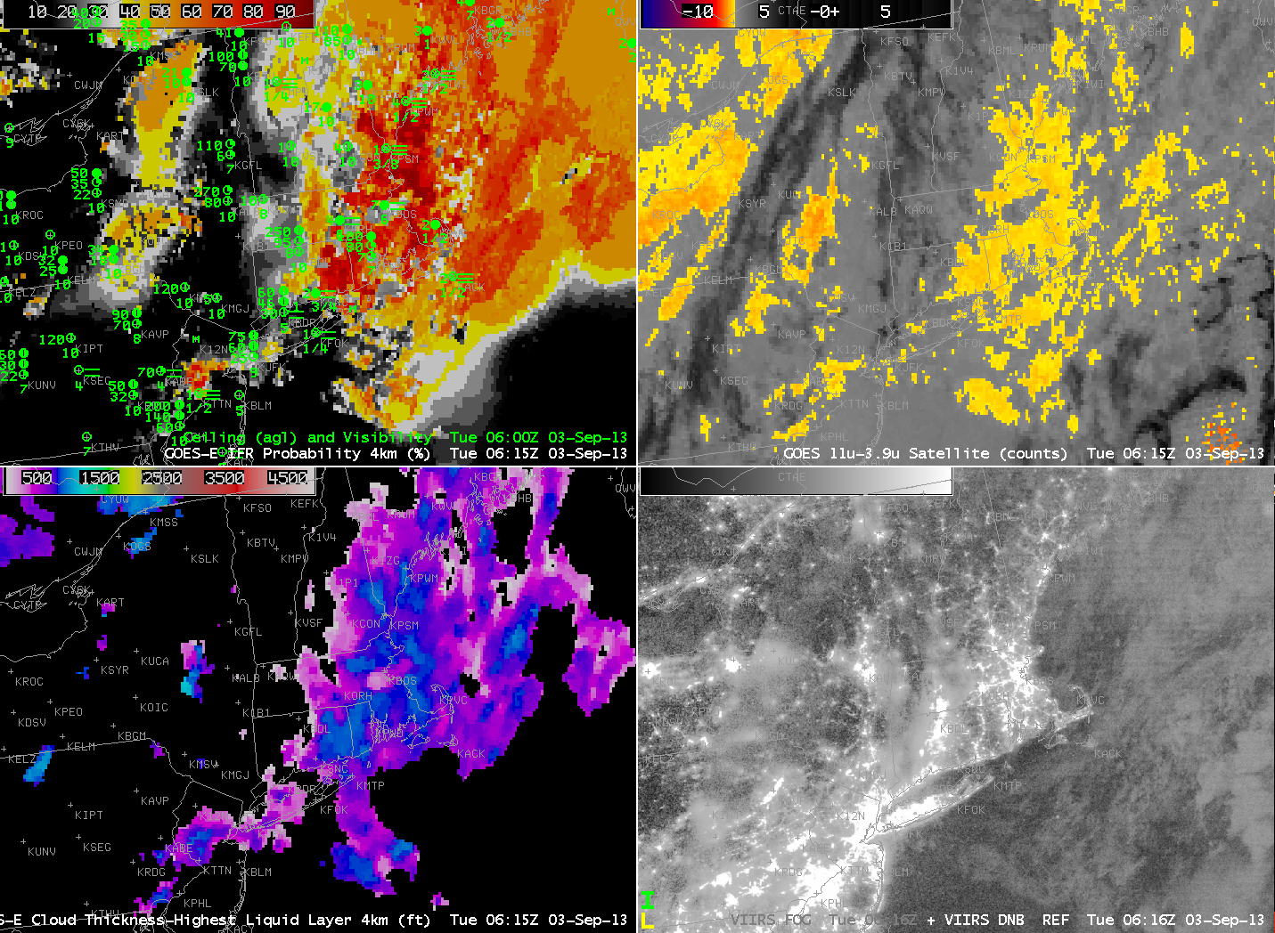
GOES-15-based GOES-R IFR Probabilities (Upper Left), GOES-15 Brightness Temperature Difference Product (10.7 – 3.9 ) (Upper Right), Color-shaded topographic map (Lower Left), GOES-15 Visible imagery and Suomi/NPP Day/Night Band (Lower Right), all times as indicated (click image to enlarge)

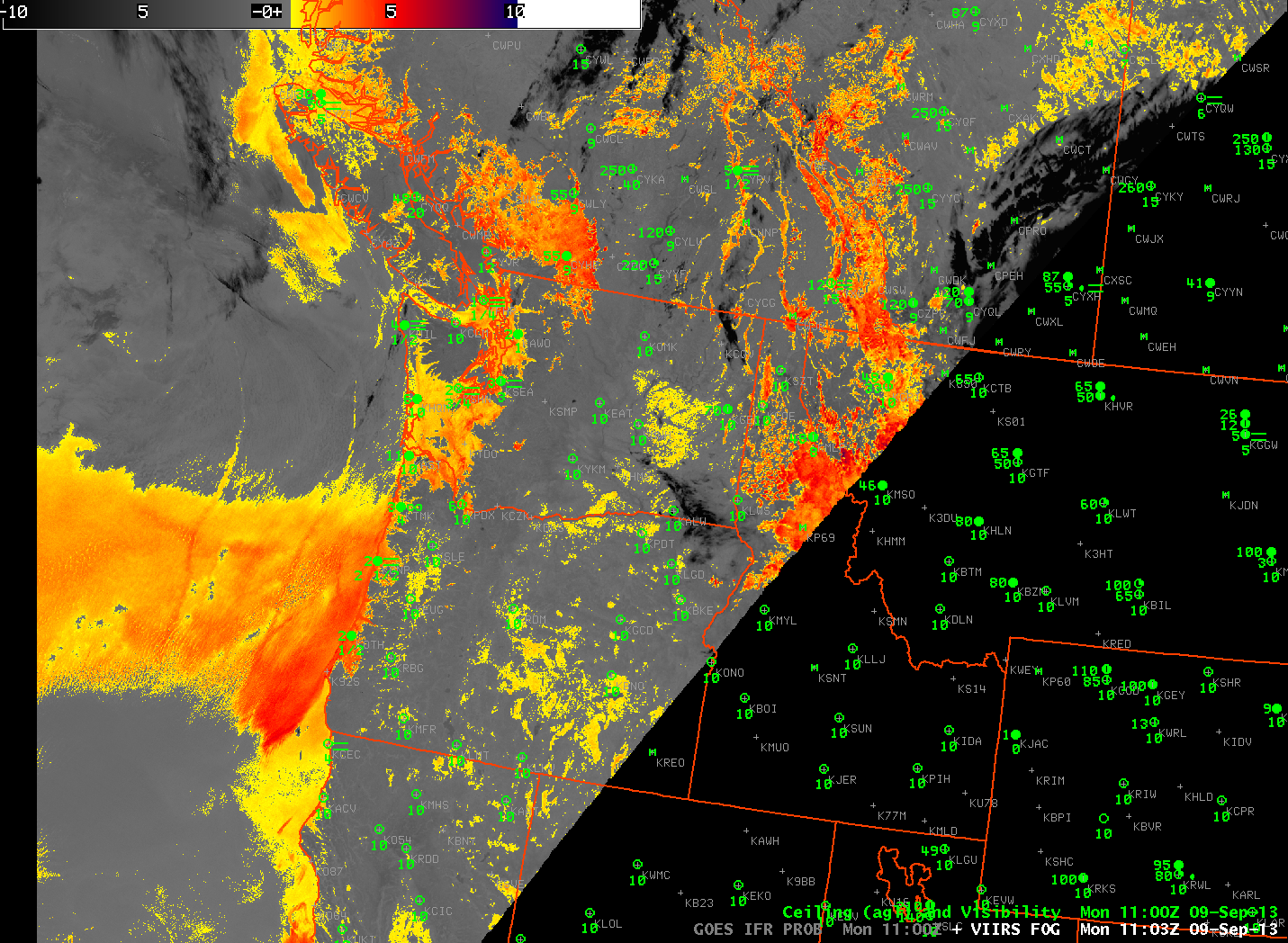
A strong low pressure system — the first strong system of the Fall Season — has made landfall along the Pacific Northwest Coast, and it provides an opportunity to see how GOES-R IFR Probabilities perform with extratropical systems.

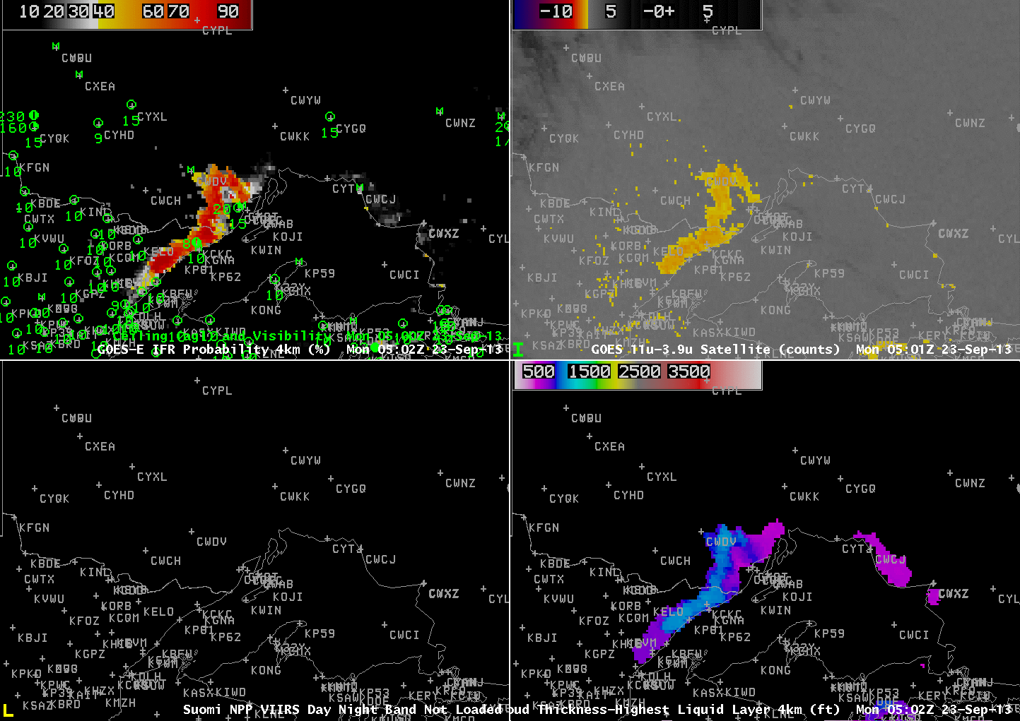
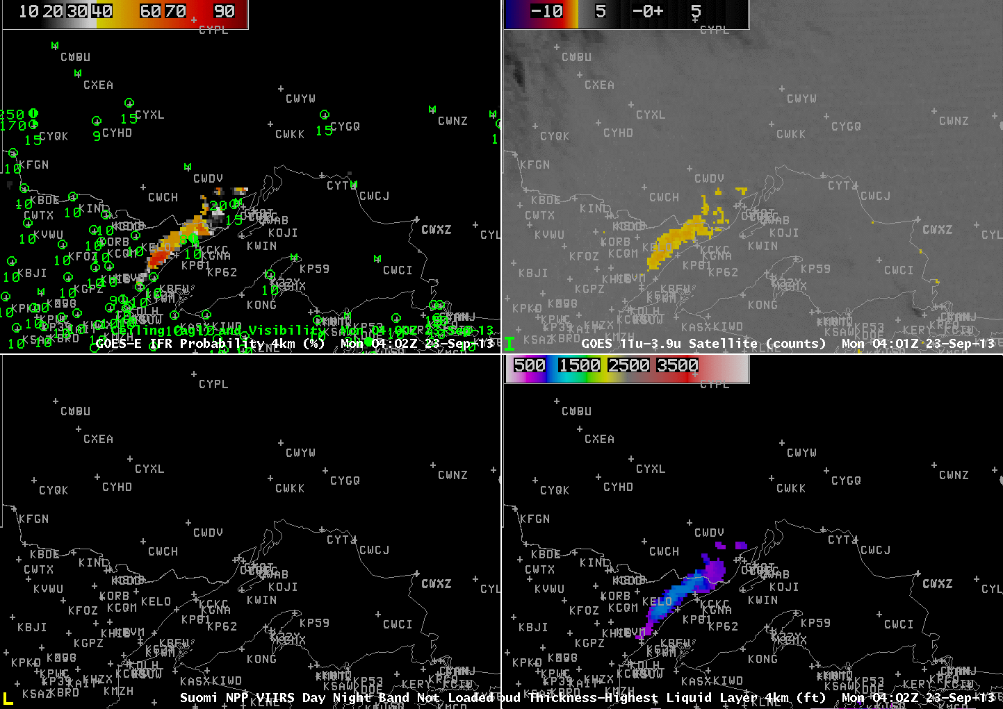
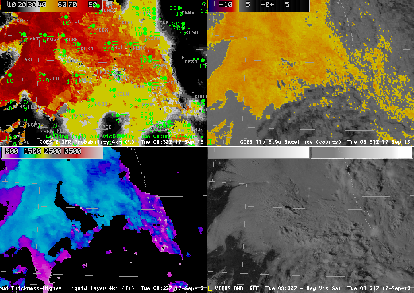
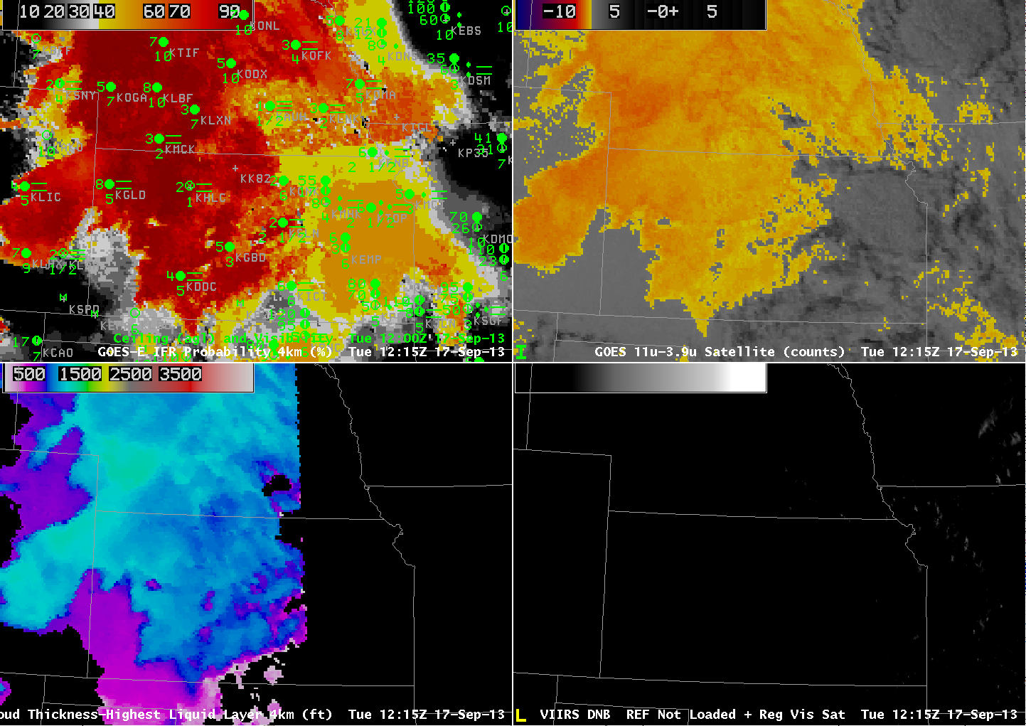
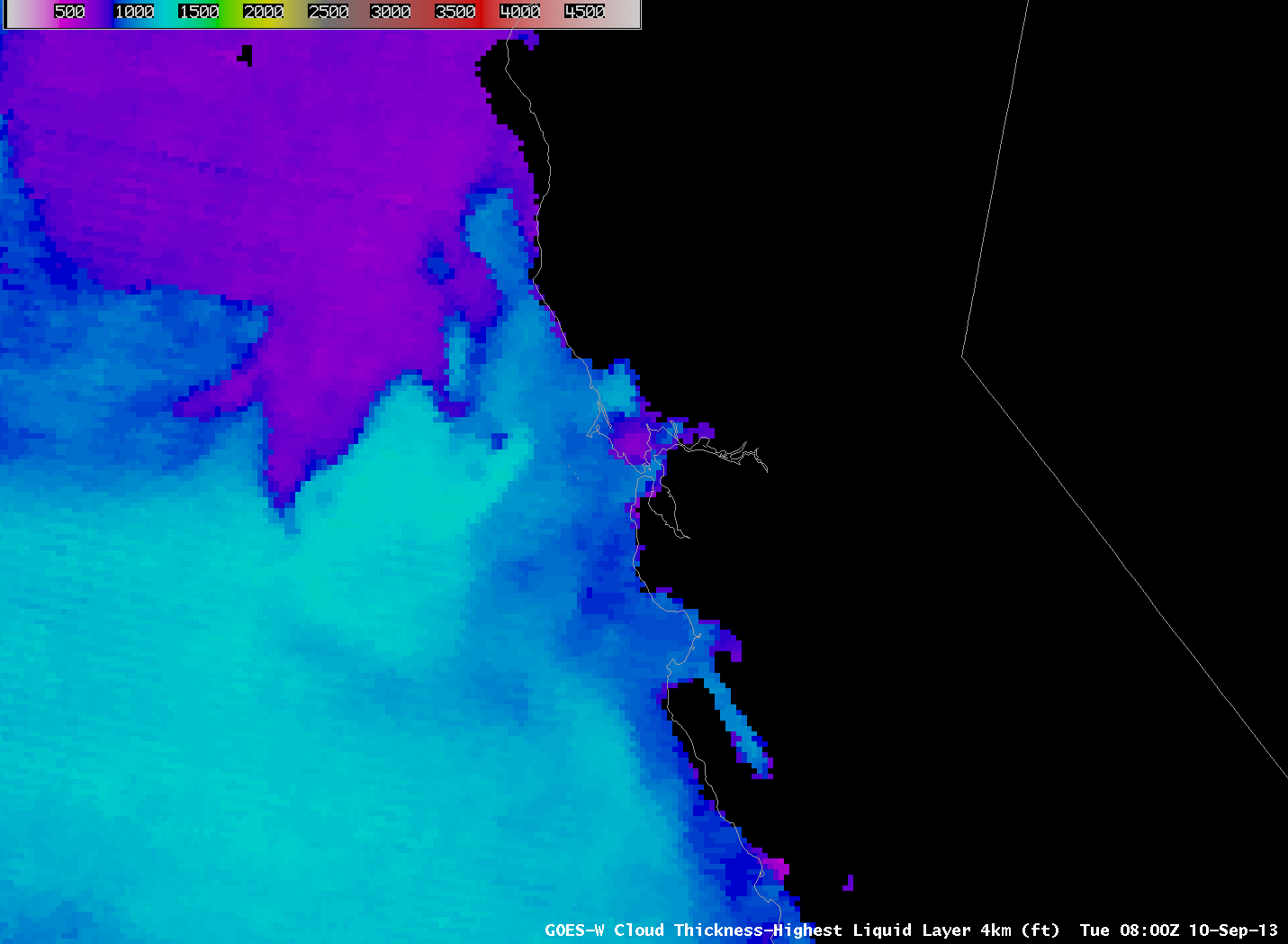
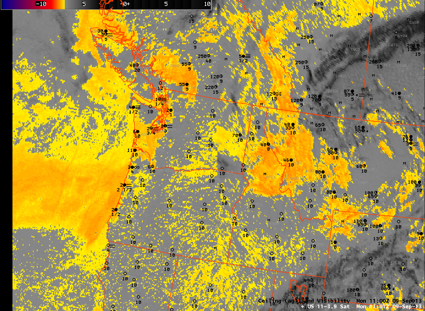
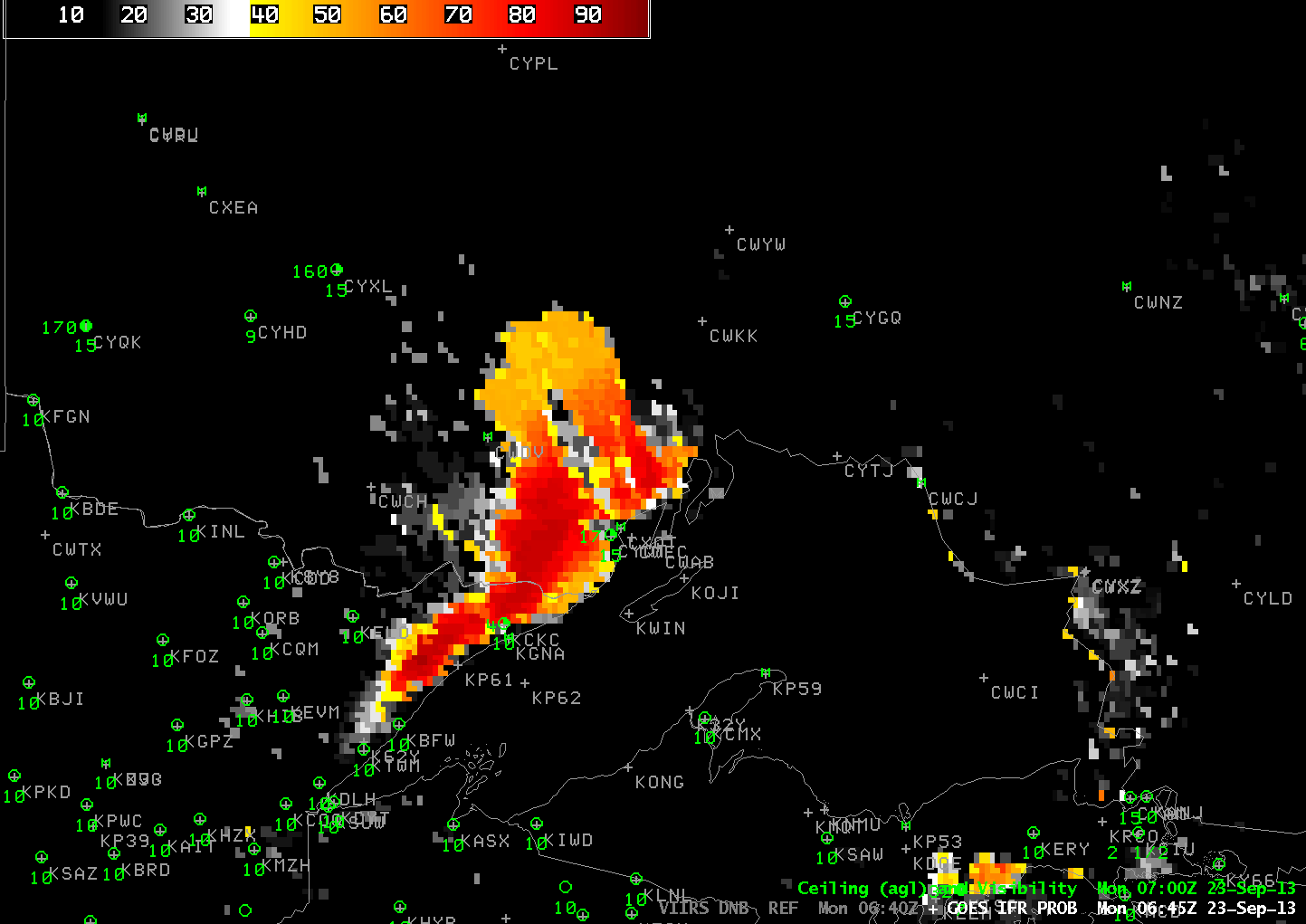
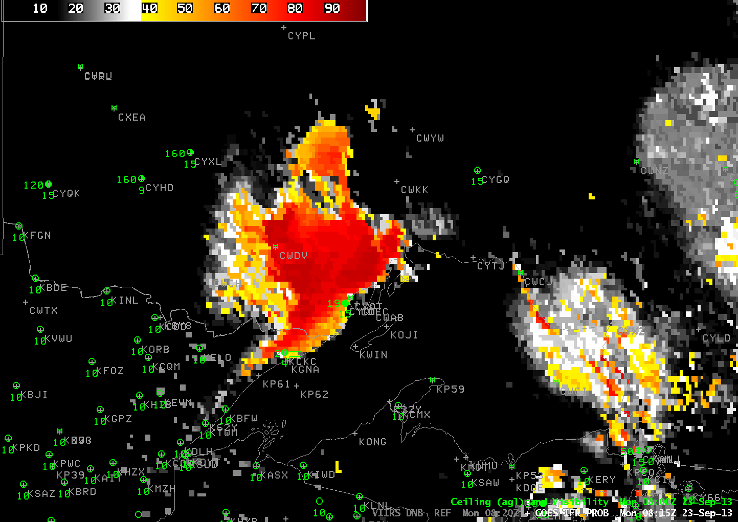
Several aspects of the IFR Probability Fields — which are far more coherent than the Brightness Temperature Difference fields — require explanation. There is an increase in the IFR Probability off the coast of Oregon in the 4th image in the loop. This jump — from IFR Probabilities near 55% (orange) to Probabilities near 68% (darker red-orange) — is likely caused by a changed in the Rapid Refresh model output that is suggesting a greater likelihood of low-level saturation. Note that this region in the very next image displays the characteristic signature of the boundary between day-time predictors being used and night-time predictors being used (IFR Probabilities drop from orange yellow — 39%). In the early part of the animation, the IFR Probability field off the Oregon Coast maintains the flat (un-pixelated) look that is characteristic of a region where only Rapid Refresh model output is being used in the computation of IFR Probabilities because high cloud are present. GOES-R Cloud Thickness (of the highest water-phase cloud, not shown) would not be computed in this region, then, for two reasons: ice and mixed-phase clouds are present and it is during twilight conditions.

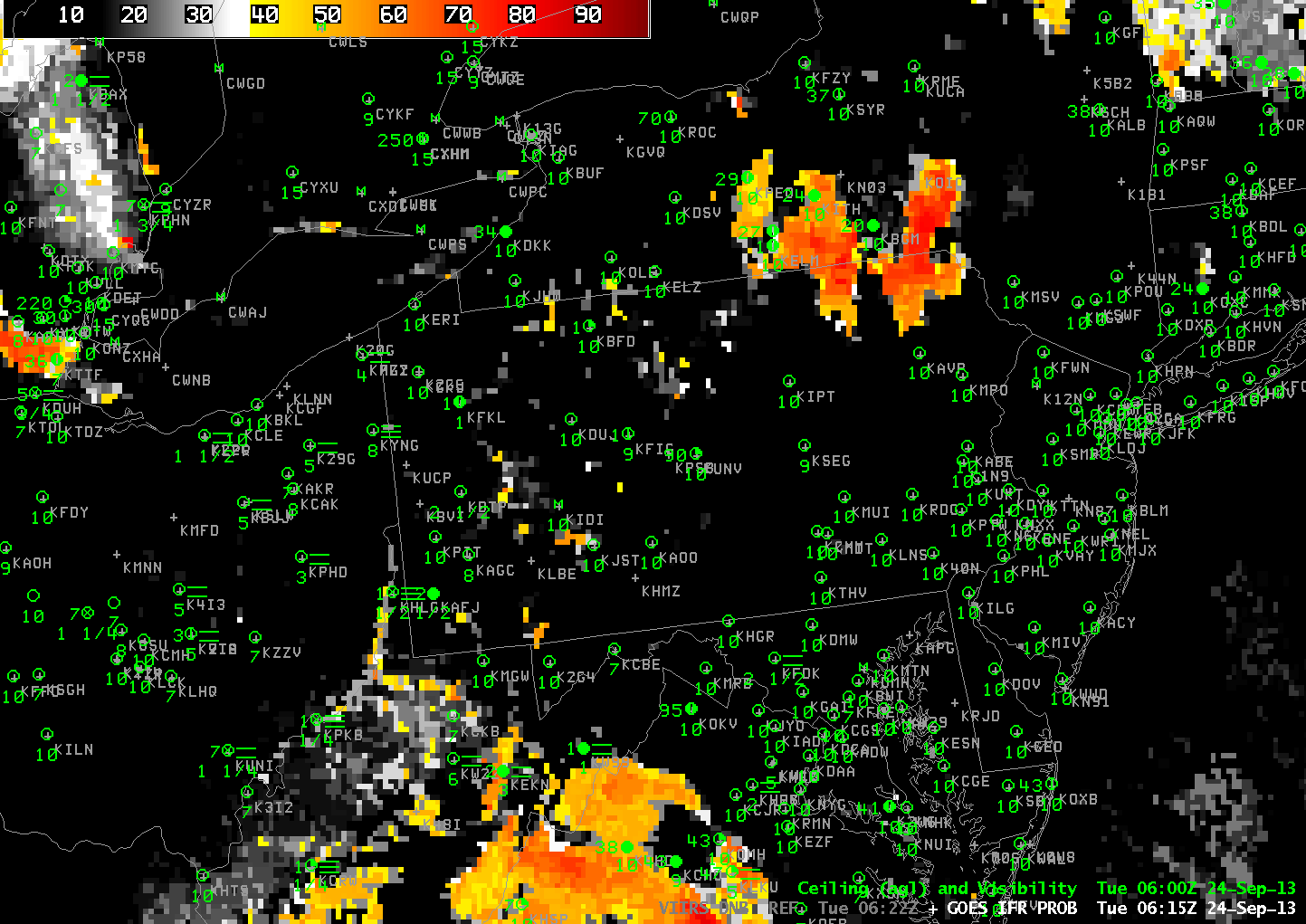
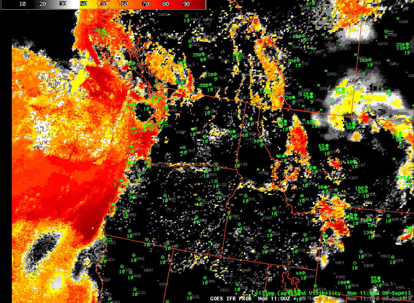
IFR and near-IFR Conditions are observed along the coast at Newport and North Bend before the frontal passage. IFR Probabilities are high along the coastal range, somewhat reduced in the Willamette Valley, high again in the Cascades, and lower again downstream of the Cascades. Note how the higher IFR Probabilities do take into account the presence of terrain; brightness temperature difference fields use only satellite data. Thus, after the frontal passage, when near-surface winds are west and south-west (that is, upslope), the IFR Probabilities remain high on the windward side of mountain slopes. (They are typically high, for example, at Sexton Summit — over KSXT — where IFR conditions are present until about 1100 UTC)

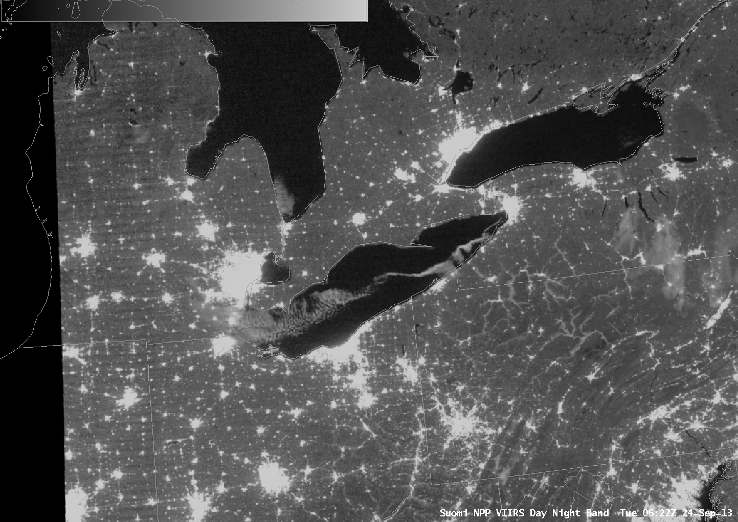
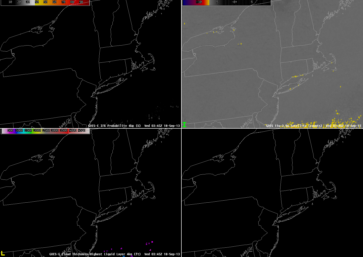
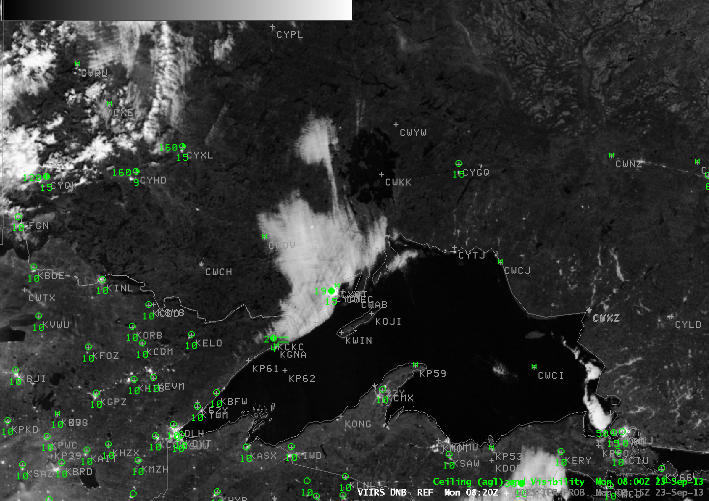
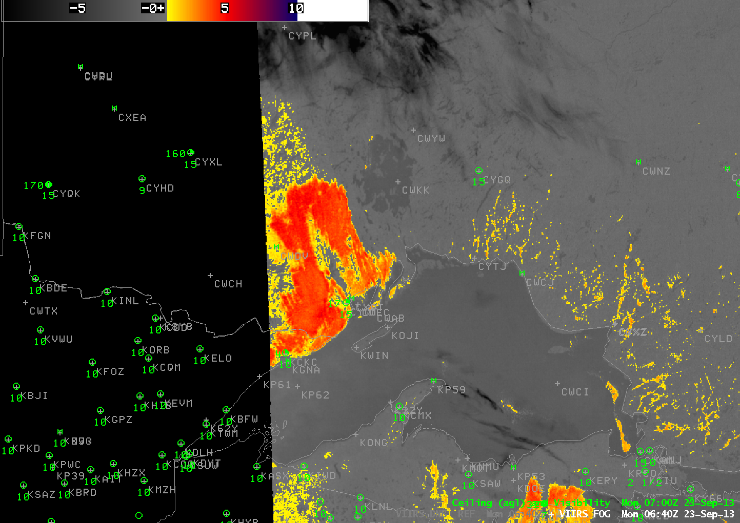
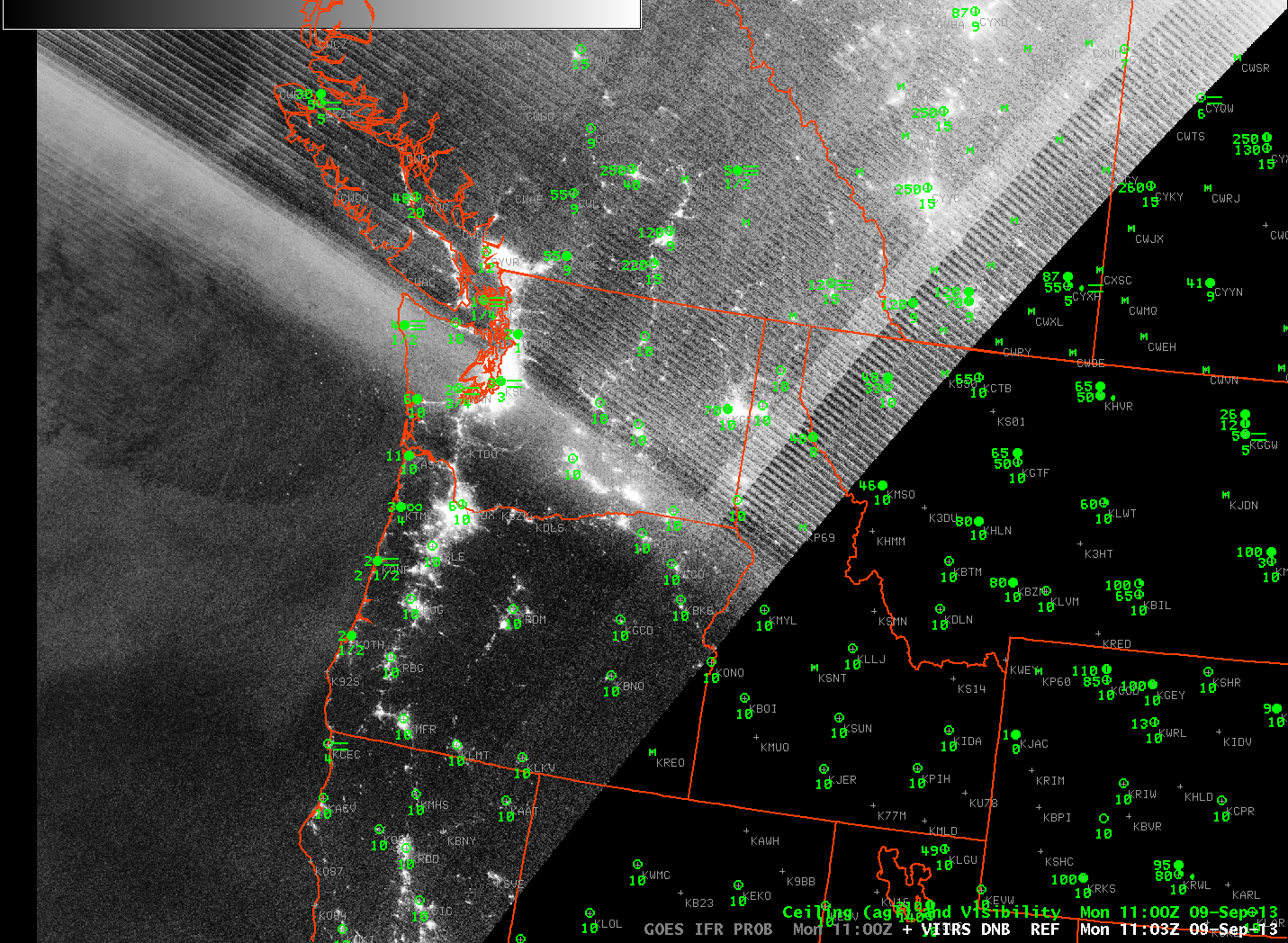
Suomi-NPP Day/Night band data can sometimes be used to discern regions of cloudiness. However, the Moon Phase is now a waning crescent that has not quite risen at the times shown in the animation above.

Resolution and Valleys

GOES_IFR_PROB_20130924_0345

GOES-based GOES-R IFR Probabilities, 0345 UTC 24 September 2013 (click image to enlarge)

Consider the GOES-R IFR Probabilities computed from GOES-East data (and Rapid Refresh data) above. How confident are you that, at 0345 UTC, fog is forming in river valleys of western Pennsylvania? Is the likelihood the same in the southern part of the state (say, along the Monongahela River) as in the northern part of the state (along the Clarion or Allegheny Rivers)? GOES resolution in the infrared channels is 4 km at the sub-satellite point. In Pennsylvania, resolution is degraded to 5 or so kilometers. The knowledge of pixel size should color your interpretation of the GOES-R IFR Probabilities (and of the brightness temperature difference field computed from GOES). The MODIS-based GOES-R IFR Probabilities from 0339 UTC, below, show a ribbon of high probabilities over many of the river valleys of Pennsylvania. This 1-km resolution information is handy at capturing the initial development of fog and low stratus.

MODIS_IFR_PROB_20130924_0339

MODIS-based GOES-R IFR Probabilities, 0339 UTC 24 September 2013 (click image to enlarge)

VIIRS_DNB__REF_20130924LakeErieLoop

Suomi/NPP VIIRS Day/Night band imagery, 0640 and 0820 UTC 24 September 2013 (click image to enlarge)

Day/Night band imagery over Pennsylvania and New York shows the expansion of fog coverage between successive Polar Passes, at 0640 and 0820 UTC. The imagery below shows the corresponding GOES-based GOES-R IFR Probabilities at those two times. The large cloud features over northeast Pennsylvania and the Southern Tier of New York are captured well by the GOES-based fields; the river valley fogs are not captured quite so well because of resolution limitations.

GOES_IFR_PROB_20130924loop

GOES-based GOES-R IFR Probabilities, 0645 and 0815 UTC 24 September 2013 (click image to enlarge)

A MODIS-based IFR probability field, below, far better represents the presence of River Valley fogs at 0746 UTC than the GOES-based IFR Probability Field, bottom, from 0745 UTC. (These times are between the two times in the GOES-R IFR Probability animation above) A good method for monitoring fog would incorporate the fine spatial resolution at the start of the fog event to ascertain which river valleys are starting first to become fog-bound. The good temporal resolution of GOES data is then used to outline the evolution of the event. Periodic Polar Orbiter passes from Terra, Aqua of Suomi/NPP as the fog event is occurring can confirm the GOES-based predictions of the evolution of fog.

MODIS_IFR_PROB_20130924_0746

MODIS-based GOES-R IFR Probabilities, 0746 UTC 24 September 2013 (click image to enlarge)

GOES_IFR_PROB_20130924_0745

GOES-based GOES-R IFR Probabilities, 0745 UTC 24 September 2013 (click image to enlarge)

Day/Night Band Imagery of Fog near Lake Superior

VIIRS_DNB__REF_20130923loop

Suomi/NPP VIIRS Day/Night Band Visible Imagery, 0640 and 0820 UTC 23 September 2013 (click image to enlarge)

The orbital geometry of Suomi/NPP is such that one geographic region will be scanned on two successive polar passes, about 90 minutes apart. The likelihood that this will happen increases as you approach the Poles. On the morning of 23 September, 2013, western Lake Superior was thus viewed twice as fog developed. This was also a night shortly after a Full Moon so ample lunar illumination allowed for a distinct view of the evolution of the fog. The 0645 UTC Day/Night band imagery shows what appears to be a much thinner cloud bank over the far northeast Minnesota Arrowhead. By 0820 UTC the cloud bank has a thicker look. Note the corresponding changes in sky/visibility at Thunder Bay (CYQT) and Grand Marais (KCKC).

VIIRS_FOG_20130923loop

Suomi/NPP Brightness Temperature Difference (11.35 µm – 3.74 µm) at 0640 and 0820 UTC, 23 September 2013 (click image to enlarge)

The Brightness Temperature Difference product can be used to identify regions of fog/low clouds. Clouds comprised of water droplets have different emissivity properties at short and long infrared wavelengths. That is, clouds do not emit as a blackbody at wavelengths around 3.74 µm; they do emit more like a blackbody at wavelengths near 11.35 µm. Thus, a brightness temperature difference from Suomi/NPP, 11.35 µm – 3.74 µm, will be warm in regions where clouds comprised of water droplets exist. In the example above, note that the brightness temperature difference is much warmer (a maximum of 5.5 K) at 0640 UTC than at 0820 UTC (where the maximum is only 4K). Why is there a difference in the two scenes?

The view at 0640 UTC is along the edge of the Suomi/NPP scan, and therefore the scan traverses a longer stretch of atmosphere, allowing for more signal absorption. Both the 3.74 µm and 11.35 µm I-Bands (the purple lines in the linked-to images) on VIIRS are broad, meaning they sense photons over a relatively large part of the electromagnetic spectrum (compared to the M-bands and to MODIS). Note that the relative response suggests that a longer pathlength through the atmosphere will cause more attenuation for the 11.35 µm channel, meaning a colder temperature. This would likely diminish the difference between the longwave and shortwave IR imagery. The opposite effect is occurring here — the brightness temperature difference is smaller in the 0820 UTC image. Why? The answer can be found in the cirrus shield impinging upon western Lake Superior in the second image. Even though the cirrus is thin, it’s radiative effect is such that the brightness temperature difference decreases.

GOES_VIIRSloop_20130923

Loop of Suomi/NPP VIIRS Day/Night Band, VIIRS Brightness Temperature Difference (11.35 µm – 3.74 µm) and GOES-East-based GOES-R IFR Probability from ~0640 and ~0820 UTC on 23 September (click image to enlarge)

How does the GOES-R IFR Probability change in the time between the two Suomi/NPP overpasses? The loop above cycles between the Day/Night Band and the Brightness Temperature Difference (from VIIRS) and the GOES-Based IFR Probability at 0645 and 0815 UTC. Highest IFR Probabilities do exist in regions where VIIRS Day/Night Band imagery and Brightness temperature difference suggest the presence of fog — between Grand Marais and Thunder Bay, and in the river valleys northeast of Lake Superior. (Poor GOES Resolution northeast of Lake Superior hampers a precise identification of where the Valley Fog is). Note that the high values of GOES-IFR probability along the Lake Superior Lakeshore, especially those lakeshores that are oriented north-south, likely stem from the coregistration error between the 3.9 µm and 10.7 µm channels on GOES-13.

GOES_IFR_PROB_20130923loop

GOES-R IFR Probability for three times centered on 0515 UTC 23 September 2013 (click image to enlarge)

The GOES-R IFR Probability shows there is still Stray Light occasionally (in the present case, at 0515 UTC only) that will contaminate the brightness temperature difference signal, and therefore also the GOES-R IFR Probability signal. A longer loop of GOES-R IFR probability, below, shows the slow expansion of IFR Probabilities during the course of the night. It also shows the effect, later in the loop, of cirrus impinging on the western shoreline of Lake Superior. IFR Probabilities drop in regions where Cirrus Clouds preclude the use of satellite data in the determination of IFR Probabilities. In addition, GOES-R Cloud Thickness is not computed in regions where cirrus clouds are present.

GOES_IFR_PROB_20130923longloop

GOES-R IFR Probability (Upper Left), GOES-East Brightness Temperature Difference (Upper Right), Suomi/NPP Day/Night Band (Lower Left), GOES-Based GOES-R Cloud Thickness (Lower Right), Times as indicated in imagery (click image to enlarge)

Brightness Temperature Differences over the Rockies

GOESVIIRS_20130919_0930

The heritage brightness temperature difference method of detecting fog/low stratus works because clouds that are comprised of liquid water droplets have different emissivity properties at 3.9 µm and at 10.7 µm. Clouds are not black-body emitters at 3.9 µm; they are more closely blackbody emitters at 10.7 µm. Consequently, the 3.9 µm radiance detected by the satellite suggests a cooler emitting blackbody temperature than the 10.7 µm radiance detected by the satellite. The difference between those two temperatures therefore highlights water-based clouds.

Some soils over the western US also have emissivity properties that are a function of wavelength such that the brightness temperature difference product will show a maximum in some regions but not in others. A careless interpretation of the brightness temperature difference signal, then, might lead to an erroneous assumption that fog/low clouds are present in a region of clear skies. The loop above shows the brightness temperature difference field at 0930 UTC on 19 September, and there are many regions with a signal that is consistent with fog/low clouds. The GOES-R IFR Probability algorithm correctly screens out many of these regions because the Rapid Refresh data does not predict low-level saturation. The day-night band image from Suomi/NPP can be used to verify where low clouds are present, and the image shows that most of the western US was clear. The IFR Probability field has false positives in 4 locations: extreme northeastern Arizona, Northwestern Mexico just to the east of the Colorado River, and two patches in the Pacific, one west of northern California, and one west of southern California.

Brightness Temperature Difference signals sometimes show positives over the central and eastern US in cases of extreme drought, as shown here.

GOES Resolution might miss valley fog (Plus: What does Stray Light look like?)

GOES_IFR_PROB_20130918_0615

GOES-R IFR Probability (Upper Left), GOES-East Brightness Temperature Difference (Upper Right), Suomi/NPP Brightness Temperature Difference (Lower Left), MODIS-based IFR Probability (Lower Right), all imagery at 0615 UTC on 18 September 2013 (click image to enlarge)

Nominal GOES resolution for the Brightness Temperature Difference product that is used in the GOES-R IFR Probability is 4 km at the sub-satellite point, and it worsens as you move into mid-latitudes. Rapid Refresh Model resolution is even coarser than the satellite. When fog is forming in narrow valleys, then, there can be a significant lag in the time from when it starts to form to when the satellite data, and the satellite/model fused product, detects it. In the 0615 UTC image above, for example, only a few pixels of strong GOES-detected Brightness Temperature Difference, and enhanced IFR Probabilities, exist. In the 0630 UTC image, below, there has been little change in the GOES-based imagery. However, the Suomi/NPP data at the time, at 1-km resolution, suggests fog is forming in many of the river valleys of Pennsylvania, but it is still sub-gridscale as far as GOES can detect.

VIIRS_DNBBTD_20130918_0634loop

GOES-R IFR Probability (Upper Left), GOES-East Brightness Temperature Difference (Upper Right), Toggle between Suomi/NPP Day/Night band imagery and Suomi/NPP Brightness Temperature Difference (Lower Left), MODIS-based IFR Probability (Lower Right), all imagery at ~0630 UTC on 18 September 2013 (click image to enlarge)

GOES_IFR_PROB_20130918_0645

GOES-R IFR Probability (Upper Left), GOES-East Brightness Temperature Difference (Upper Right), Suomi/NPP Brightness Temperature Difference (Lower Left), MODIS-based IFR Probability (Lower Right), all imagery at 0645 UTC on 18 September 2013 (click image to enlarge)

Fifteen minutes later, the MODIS-based IFR probabilities (above) suggest a strong possibility of IFR conditions in many of the river valleys of Pennsylvania. However, Suomi/NPP and MODIS data come from polar orbiters so that high resolution information is infrequent. When GOES-R is launched, ABI will have nominal 2-km resolution in the infrared, which resolution is intermediate between GOES and MODIS.

The higher-resolution polar orbiters’ occasional views can give a forecaster an important heads’ up for fog formation. By 0815 UTC the GOES-based information is showing higher IFR probabilities in the river valleys of Pennsylvania, but a Suomi/NPP overpass shows that it is still underestimating the areal extent of the fog.

VIIRS_DNBBTD_20130918_0817loop

GOES-R IFR Probability (Upper Left), GOES-East Brightness Temperature Difference (Upper Right), Toggle between Suomi/NPP Day/Night band imagery and Suomi/NPP Brightness Temperature Difference (Lower Left), MODIS-based IFR Probability (Lower Right), all imagery at ~0815 UTC on 18 September 2013 (click image to enlarge)

Note that this is a time of year when stray light does occasionally enter the GOES signal, causing contamination. This occurred — and was very obvious — around 0400 UTC on 18 September. As is typical, it was present for only one scan. See below.

GOES_CLD_THICK_20130918loop

GOES-R IFR Probability (Upper Left), GOES-East Brightness Temperature Difference (Upper Right), GOES-R Cloud Thickness (Lower Left), MODIS-based IFR Probability (Lower Right), all imagery at ~0815 UTC on 18 September 2013 (click image to enlarge)

Fog over Kansas

GOES_IFR_PROB_20130917_0832

GOES-R IFR Probability (Upper Left), GOES-East Brightness Temperature Difference (Upper Right), GOES-R Cloud Thickness (Lower Left), Suomi/NPP Day/Night Band (Lower Right), all imagery at ~0830 UTC on 17 September 2013 (click image to enlarge)

Light winds with a small upslope component allowed for the formation of fog over the High Plains on the morning of 17 September 2017. The image above shows the GOES-R IFR Probability, GOES-East Brightness Temperature Difference (10.7 µm – 3.9 µm), the GOES-R Cloud Thickness and the Day/Night band from Suomi/NPP that provides for nighttime visible imagery. In the imagery above, a large region over southeastern Kansas is overlain by higher ice-based clouds (likely cirrus) such that the brightness temperature difference product does not give the signal that is common with fog and low stratus (in the enhancement used here, fog and low stratus occur where the brightness temperature difference is colored orange or yellow). The Day/Night band visible imagery also suggests high clouds over southeast Kansas. Surface observations do show reduced visibilities, at or near IFR conditions. In this region, the IFR Probability Product gives useful information by using Rapid Refresh Data to diagnose the possibility of low-level fog. The probabilities are smaller — in the 40- to 50% range — but that is because no satellite data are being used as predictors. IFR Probabilities are very high only if both predictors — satellite and Rapid Refresh — are associated with high probability of fog/low stratus.

Note also how the Cloud Thickness product yields no information where high clouds are present. The Cloud Thickness is the thickness of the highest liquid cloud layer; the presence of ice clouds or mixed phase clouds precludes the determination of how thick a water cloud is because the satellite cannot view the water-based cloud.

GOES_IFR_PROB_20130917_1215

As above, but at 1215 UTC (click image to enlarge)

The 1215 UTC image shows the effect of twilight conditions moving westward across Kansas — GOES-R Cloud Thickness is not computed during twilight conditions that occurring over eastern Kansas, although they are still computed around Dodge City, where the computed cloud thickness is just over 1000 feet thick. The 1200 UTC Sounding from Dodge City, below, does show a nearly-saturated layer at the surface (about 927 mb, or about 2700 feet ASL) up to about 870 mb (4600 feet ASL).

KDDC_20130917_1200

Upper Air Sounding from Dodge City, KS, 1200 UTC (click image to enlarge)

GOES-15 Navigation Anomalies

GOES_CLD_THICK_20130910navloop

GOES-R IFR Cloud Thickness computed from GOES-West and Rapid Refresh data (click image to enlarge)

For the past 3 mornings (8, 9 and 10 September) GOES-15 Navigation has suffered an anomaly around 0930 UTC. The animation above shows the effects: Cloud Thickness fields (and IFR probability fields, not shown) are shifted. Click here for more information. The navigation anomalies typically end around 1030 UTC.

Fog/Low Clouds over the Northwestern US

GOESBTD_IFR_20130909_1100

Brightness Temperature Difference from GOES-W and GOES-R IFR Probability computed from GOES-West and Rapid Refresh data, both images at 1100 UTC 9 September (click image to enlarge)

Fog and low clouds off the coast of Washington and in Montana are instructive in describing some strengths of the GOES-R IFR Probability algorithm. A general statement is that the IFR Probability improves — sometimes greatly — the approximation of where fog and low clouds are present. In the example above, the brightness temperature difference shows a positive signal — suggestive of low clouds — along the Washington and Oregon coasts (where IFR conditions are reported within the marine layer of stratus/fog). The brightness temperature difference also has a strong signal over Montana; there is a scattershot signal as well over Nevada, Idaho and western Oregon/Washington. These are regions where the GOES-R IFR Probability field is correctly minimizing the probability of fog/low clouds. Over Montana, the Brightness Temperature Difference signal is driven by an elevated stratus deck. The positive signal in arid Nevada, Idaho, Oregon and Washington arises from soil emissivity variability. The IFR Probability field maintains a strong signal where IFR conditions are reported, and reduces the strong signal in regions where fog/low stratus likely do not exist.

BTD_GOES_VIIRS_20130909_1100

Brightness Temperature Difference from GOES-W and and from Suomi/NPP, both images at ~1100 UTC 9 September (click image to enlarge)

Suomi/NPP was passing over the Pacific NW at 1100 UTC, the times of the imagery above, and it provided a higher-resolution look. Suomi/NPP data allows for better definition of the — apparently — thickest stratus/fog layer right along the Washington and Oregon coast. The superior resolution also allows for a better approximate of the dendritic nature of river valley clouds, as demonstrated over southern British Columbia. However, the brightness temperature difference here is also unable to distinguish between fog on the ground and stratus that at mid levels.

PacNW_FOG_20130909_1100

Brightness Temperature Difference from GOES-W, Day/Night Band, Brightness Temperature Difference from Suomi/NPP, Day/Night Band, GOES-based GOES-R IFR Probabilities, all at ~1100 UTC 9 September (click image to enlarge)

The animation above loops through the GOES-Based Brightness temperature difference, the Suomi-NPP Brightness temperature difference, the Suomi-NPP Day/Night band, and the GOES-R IFR Probability field computed with GOES-W and Rapid Refresh data.

IFR Conditions over southwest Alaska

GOES_IFR_PROB_20130905loop

GOES-R IFR Probability computed from GOES-West (click image to play animation)

A relatively narrow band of high IFR probabilities developed over southwest Alaska, as shown in the animation above. Pay particular attention to the observations at St. Marys (PASM) and at Emmonak (PAEM). These two stations have near-IFR and IFR conditions as the high IFR Probability develops and curls over them.

alaska_11-3.9_Sat_20130905loop

GOES-West Brightness Temperature Difference Field (click image to play animation)

The traditional method of detecting fog and low clouds, the brightness temperature difference between the 10.7 and 3.9 micrometer channels, does not distinguish between the region with IFR conditions and adjacent regions. Adding information from the Rapid Refresh model in this case fine-tuned the depiction of where the greatest restrictions to visibility exist.

Suomi-NPP Brightness temperature difference fields (below) had a similar deficiency in precisely highlighting the region with IFR conditions.

VIIRS_FOG_20130905_1357

Suomi-NPP VIIRS Brightness Temperature Difference Field (click image to play animation)

Fog over southern New England

The National Weather Service in Taunton, MA, tweeted an image of fog over coastal southern New England early on September 3rd. How well did the GOES-R IFR Probability detect this event?

GOES_IFR_PROB_20130903loop

GOES-R IFR Probability (click image to play animation)

The animation, above, at hourly time-steps (GOES-R IFR Probability is computed every 15 minutes, usually, but matching surface observations occur only hourly) can be used to validate the accuracy of the IFR Probability product: highest probabilities in the animation are occurring over coastal New England where visibility is lowest. The increase in probabilities from 1002 UTC to 1102 UTC over the Gulf of Maine reflects the night-time (1002 UTC) vs. daytime (1102 UTC) predictors being used in the IFR Probability algorithm. The flat nature of the IFR probability field over parts of the Gulf of Maine suggests that model data only is being used to compute the IFR probability field there. This occurs where high clouds obscure the satellite view of low clouds.

GOES_IFR_PROB_20130903_1315loop

GOES-R IFR Probability (Upper Left), GOES-East Brightness Temperature Difference (Upper Right), GOES-R Cloud Thickness (Lower Left), Suomi/NPP Day/Night Band (Lower Right) (click image to play animation)

The brightness temperature difference fields in the animation above (click image to see the animation) have a characteristic appearance associated with high clouds south and east of Cape Cod. In fact, Nantucket is mostly overlain by high clouds. The presence of those high clouds makes satellite detection of fog/low stratus difficult, but a fused/blended product such as the GOES-R IFR probability field that combines satellite and model data is able to alert an observer to the presence of reduced visibilities.

The GOES-R Cloud Thickness (Lower left in the animation above) gives an estimate to the depth of the highest water-based cloud layer. This product is not computed during twilight conditions — from about 1015 to 1215 UTC in the animation above. The animation clearly shows the thickest fog/low stratus deck moving eastward through southeast New England during the early morning hours.

The Suomi/NPP Day/Night band allows for visible imagery at night, detecting visible moonlight and Earthglow that is reflected off clouds, and also emitted light from cities. The 0615 UTC image is here. Clouds are visible in the image, but there is no information on the level of the cloud.

GOES_EAST_3SEP2013loop

GOES-13 Visible Imagery (click image to play animation)

Visible imagery from after sunrise shows the low clouds persisting south of New England. In addition, a bore (manifest as a series of parallel lines) propagates south of an area of convection that appears to have spawned the bore.