Monthly Archives: October 2016

IFR Conditions over the Deep South

GOES-R IFR Probability Fields, 0100-0500 UTC on 31 October 2016 (Click to enlarge)

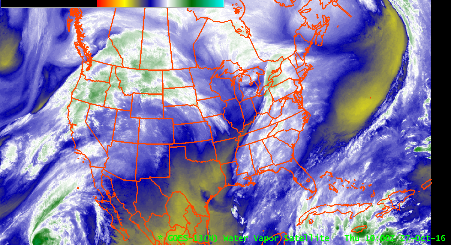
GOES-13 Brightness Temperature Difference Fields (3.9 µm – 10.7 µm), 0100-0500 UTC on 31 October 2016 (Click to enlarge)

Compare the two animation from 0100-0500 above, showing GOES-R IFR Probability fields (top) and GOES-13 Brightness Temperature Difference fields (bottom) from shortly after sunset on 30 October 2016 until Midnight. IFR Probability shows very little signal at first, and IFR conditions are rare (Jack Edwards Airport near Gulf Shores AL report IFR conditions). IFR Probabilities increase slowly in the next 4 hours, especially in regions where IFR conditions develop. In contrast, the trend in the Brightness Temperature Difference field is a slow decrease in areal coverage with little spatial correlation between a strong signal and IFR reports. These animations demonstrate a strength of IFR Probabilities: By combining satellite information with Rapid Refresh predictions of low-level saturation, a better estimate of visibility restrictions can be created.

Subsequent to 0500 UTC, in the animations shown below, IFR Probability fields expanded as IFR conditions developed over western Louisiana and southern/eastern Texas; a strong signal develops in the brightness temperature difference field in these regions as well. Note the lack of signal in the GOES-R IFR Probability field over Alabama and Mississippi where Brightness Temperature Difference fields show a consistent signal (and where IFR Conditions are not present). Brightness Temperature Difference signals over those states may be related to changes in emissivity properties that occur during severe drought, as discussed here.

GOES-R IFR Probability fields, 0500-1215 UTC on 31 October 2016 (Click to enlarge)

GOES-13 Brightness Temperature Difference Fields (3.9 µm – 10.7 µm), 0500-1215 UTC on 31 October 2016

GOES-R Cloud Thickness relates future dissipation of fog to present observations of Cloud Thickness. The last pre-sunrise GOES-R Cloud Thickness field is related to dissipation time in this scatterplot. (GOES-R Cloud Thickness is not computed during twilight times surrounding sunrise and sunset) The animation below shows the thickest clouds over south-central Texas; fog over Louisiana and coastal Texas is comparatively thin. Dissipation should occur last over interior Texas.

goes-rcloudthickness_1145-1245_31oct2016step

GOES-R Cloud thickness every half hour from 1145-1245 UTC on 31 October 2016 (click to enlarge)

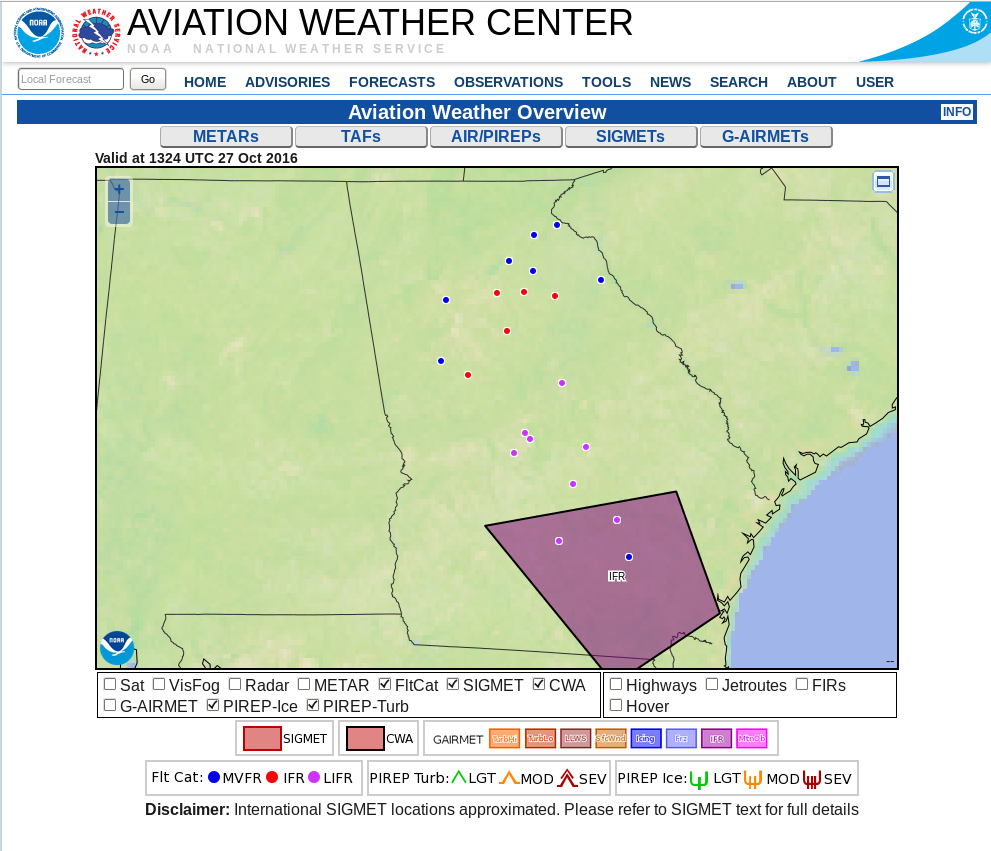
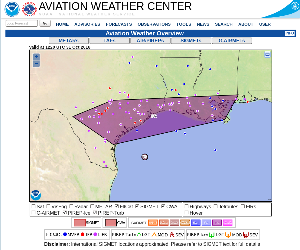
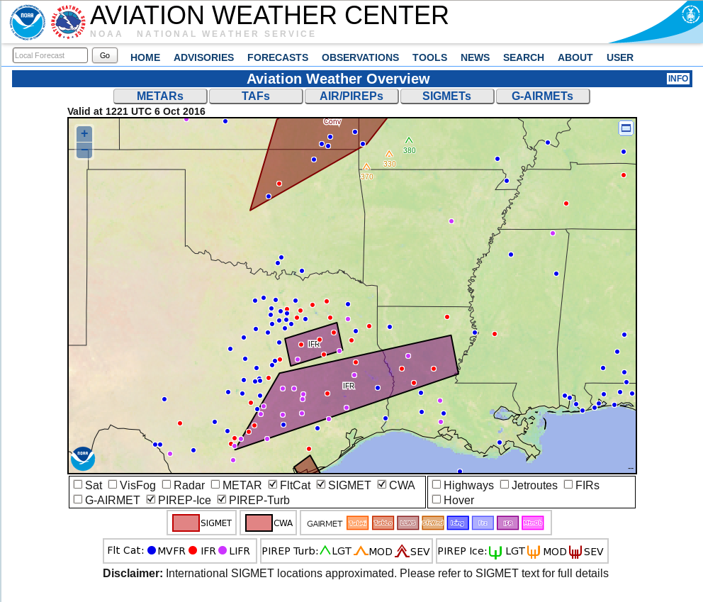
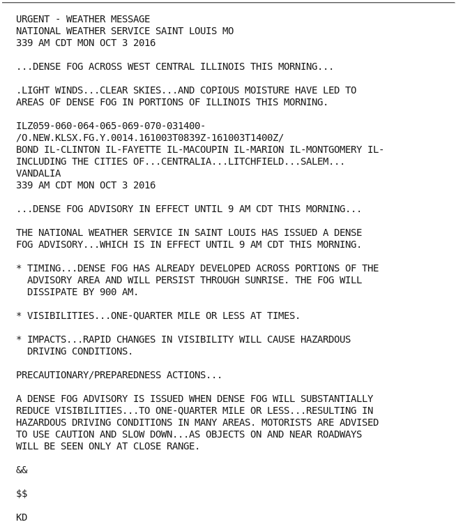
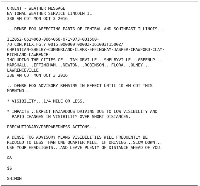
IFR probabilities were noted by the Aviation Weather Center, and Dense Fog Advisories were issued along the Gulf Coast for this case.

IFR Probability Fields let you peek beneath the Cirrus

GOES-13 Brightness Temperature Difference (3.9 µm – 10.7 µm) fields, hourly from 0215-1215 UTC on 27 October (Click to enlarge)

If you rely on satellite data alone to anticipate the development of IFR conditions — fog, low ceilings, and reduced visibilities — then the presence of widespread cirrus, shown here with the GOES-13 6.5 µm image, makes situational awareness difficult. At a glance, can you tell in the animation of brightness temperature difference, above, hourly from 0215 through 1215 UTC, where IFR Conditions are occurring? The widespread cirrus, present in the enhancement as dark grey and black, prevents the satellite from viewing any fog development, hence making this brightness temperature difference field, traditionally used to detect the development of fog and low stratus, unsuitable for large-scale situational awareness.

GOES-R IFR Probability fuses satellite data with Rapid Refresh Model output and allows a product that in essence peeks beneath the cirrus because near-surface saturation predicted in the Rapid Refresh Model allows the IFR Probability product to have a strong signal where fog might be developing. Consider the animation below, that covers the same spatial and temporal domain as the brightness temperature difference animation above. IFR Probability increases over inland southeast Georgia in concert with the development of low ceilings/reduced visibilities. It gave a few hours alert to the possibility that IFR conditions would be developing. Note in the animation below that the 1215 UTC image includes IFR Probabilities computed using daytime predictors and nighttime predictors. There is therefore a discontinuity in the field values over central Georgia at 1215 UTC, the end of the animation.

Compare the animation below to the one above. Which yields better situational awareness for the developing fog field?

GOES-R IFR Probability Fields, hourly from 0215 through 1215 UTC on 27 October (Click to enlarge)

The Aviation Weather Center plot (below) highlights the presence of an IFR SIGMET over the region at 1324 UTC on 27 October.

Aviation Weather Center plot showing MVFR, IFR and LIFR stations over Georgia, along with an IFR Sigmet at 1324 UTC 27 October 2016 (Click to enlarge)

IFR Probability Screens out mid-level Stratus

GOES-13 Brightness Temperature Difference (3.9 µm- 10.7 µm) and GOES-R IFR Probability fields computed with GOES-13 and Rapid Refresh Data, 1100 UTC 18 October. Plots of ceilings and surface visibilities are included (Click to enlarge)

GOES-R IFR Probability fields often to a better job (compared to brightness temperature difference fields) in outlining exactly where low ceilings and reduced visibilities are occurring because IFR Probability fields include information about low-level saturation from the Rapid Refresh model. That information about near-surface saturation allows the IFR Probability algorithms to screen out regions where only mid-level stratus is occurring. A low fog — a stratiform cloud of water droplets that sits on/near the surface — and a mid-level stratus deck (also a stratiform cloud of water droplets) can look very similar in a brightness temperature difference field. In the example above, consider much of northeastern Alabama and northern Georgia. There is a strong return in the brightness temperature difference field because mid-level stratus is present — but IFR Probabilities are small because the Rapid Refresh does not diagnose low-level saturation in the region. Compare Brightness Temperature Difference returns over northeast Alabama and over extreme western North Carolina — to the west of Asheville. IFR Conditions are observed over western North Carolina, and IFR Probabilities are high there. In general, the region with high IFR Probabilities in the toggle above includes stations that are reporting IFR or near-IFR conditions. Most stations outside the region of high IFR Probability are not showing IFR Conditions, even though they may be in a region with the Brightness Temperature Difference signal is large.

A similar story can be told farther west at 0800 UTC, shown below. Focus on the region with a strong Brightness Temperature Difference signal over southeast Arkansas. IFR Conditions are not occurring under that mid-level stratus deck, and IFR Probabilities are very low. Similarly, IFR Probabilities are small over Oklahoma and north-central Texas because the Rapid Refresh Model is not showing low-level saturation in those regions; IFR Probabilities cannot be large when low-level saturation is not indicated in the model.

Using both Satellite Data and Model Data accentuates the strengths of both. That’s the power of a fused data product.

GOES-13 Brightness Temperature Difference (3.9 µm – 10.7 µm) and GOES-R IFR Probability fields computed with GOES-13 and Rapid Refresh Data, 0800 UTC 18 October. Plots of ceilings and surface visibilities are included (Click to enlarge)

IFR Probability Motion as a forecast tool

GOES-R IFR Probability Fields, 0200-1400 UTC on 13 October 2016 along with surface observations of ceilings/visibility (Click to enlarge)

Because GOES-R IFR Probability fields are computed with the same time latency as GOES imagery, motion of the IFR Probability fields can have predictive value. In the animation above, higher GOES-R IFR Probability is moving eastward; IFR Conditions are reported as the higher IFR conditions move overhead (consider, for example, Bowling Green, KY, or Clarksville, TN), and ceilings / visibilities improve as the band of higher IFR conditions moves eastward from a station (over southern Illinois, for example).

IFR Probabilities over Louisiana

ifrprobability_goes13btd_1107_6oct2016toggle

GOES-13 Brightness Temperature Difference Fields and GOES-13-based GOES-R IFR Probability fields, 1107 UTC on 6 October (Click to enlarge)

The toggle above between the GOES-R IFR Probability fields at 1107 UTC on 6 October, and the corresponding Brightness Temperature Difference field from GOES-13, is an example of the strength of the GOES-R IFR Probability field. By fusing Satellite Data with model (Rapid Refresh) estimates of low-level saturation, the Probability field is able to differentiate between regions where Brightness Temperature Difference fields are showing a signal but where widespread low-level fog is not occurring (Mississippi) from regions where Brightness Temperature Difference Fields show a signal and where IFR conditions are present (Louisiana and Texas). An IFR SIGMET was issued associated with the Fog over Louisiana and Texas.

Fog over the lower Ohio River Valley

GOES-R IFR Probability Fields, 0200-0700 UTC on 3 October 2016 (Click to enlarge)

Fog developed over portions of the Ohio River Valley from Indiana westward to the Mississippi River at Cairo IL on the morning of 3 October 2016. Dense Fog Advisories were issued by the National Weather Service Offices in St. Louis, Lincoln IL and Paducah between 3:30 and 4:15 CDT (0830 to 0915 UTC). A SIGMET was also issued. How effective was Satellite detection of this developing fog?

The brightness temperature difference product, below, shows hourly measures of water-based clouds, a detection that keys off the emissivity differences of water based clouds for 3.9 radiation (at which wavelength near-blackbody emission is not occurring) and 10.7 radaiation (at which wavelength near-blackbody emission is occurring). Significant changes to the brightness temperature difference field did not occur until after 0500 UTC. In addition, Brightness Temperature Difference fields overestimated the region of developing fog. In contrast, the GOES-R IFR Probability field, above, showed a more gradual increase from 0200 UTC onward, and the region of the strong signal was better confined to where dense fog developed. On this day, GOES-R IFR Probability fields were better for situational awareness, generating an earlier alert for forecasters to the potential for fog. In addition, the GOES-R IFR Probability fields better defined the region of hazardous ceilings and visibilities.

Brightness Temperature Difference Field (3.9 – 10.7) from 0100 to 0700 UTC on 3 October 2016 (Click the enlarge)

GOES-R Fog Product Examples

Fog detection fusing GOES, Terra/Aqua or Suomi/NPP Satellite data with Model output