Monthly Archives: December 2016

Dense Fog in Oregon

GOES-R IFR Probabilities computed with GOES-15 and Rapid Refresh Data, hourly from 0300 through 1400 UTC on 21 December 2016 (Click to enlarge)

Dense Fog developed in the Willamette Valley of western Oregon during the early morning hours of 21 December 2016.  How did GOES-R IFR Probability fields and GOES-15 Brightness Temperature Difference (3.9 µm – 10.7 µm) Fields diagnose this event that led to the issuance of Dense Fog Advisories? The hourly GOES-R IFR Probability animation, above, shows increasing probabilities in the Willamette Valley, starting around Eugene (KEUG) and spreading northward until high probabilities cover the valley by 1400 UTC. IFR Conditions are first reported near Eugene, then through the entire valley by 1400 UTC. Widespread high IFR Probability values are not present elsewhere over Oregon (although they do exist over Washington State, where IFR conditions were also observed).

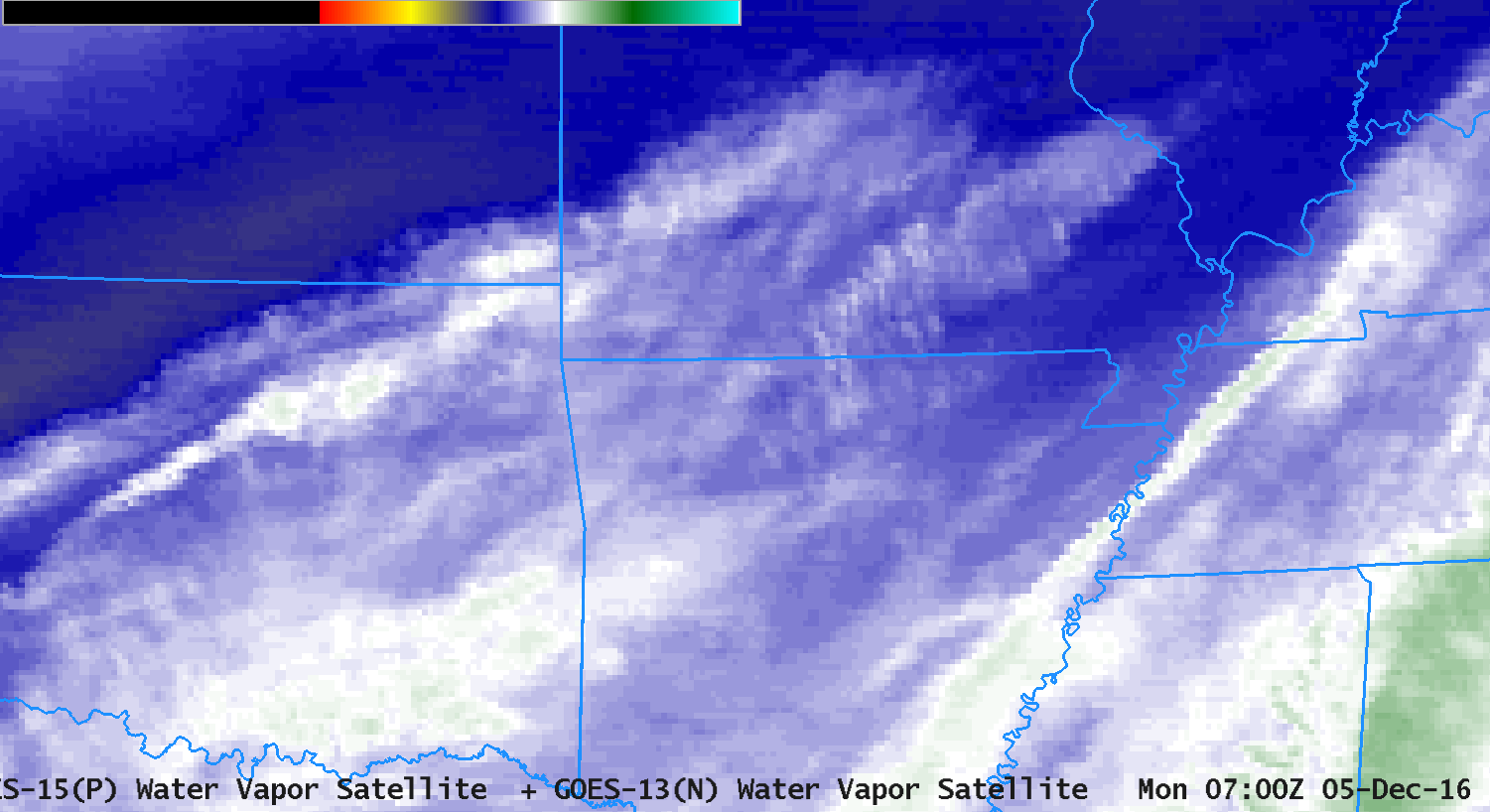
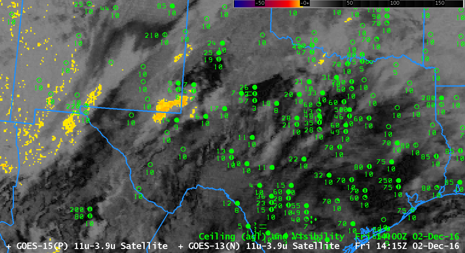
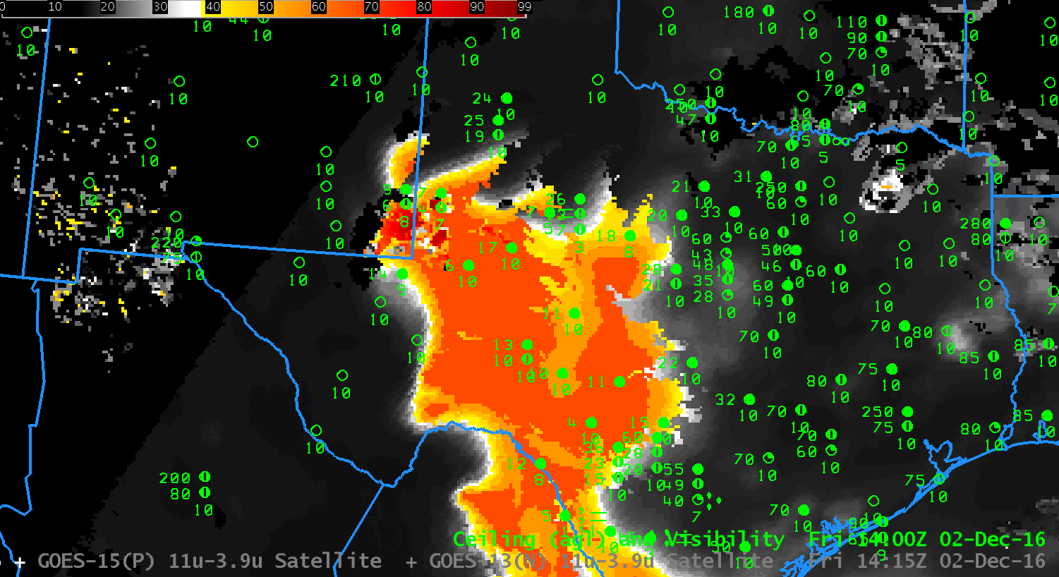
The Brightness Temperature Difference field (3.9 µm – 10.7 µm), below, shows a different distribution. Early in the animation a strong signal is apparent over much of northern Oregon, and also over the Pacific Ocean. Rapid Refresh output on low-level saturation is used in the GOES-R IFR probability algorithm to screen out regions where stratus that is detected by the satellite likely is not extending down to the surface — over the ocean, for example (coastal sites do not show IFR Conditions), or over much of eastern Oregon/Washington.   Brightness Temperature Difference fields do eventually highlight the presence of fog in the Willamette Valley, but considerable regions outside the valley have a strong return and no indication of IFR conditions.

GOES-15 Brightness Temperature Difference (3.9 µm – 10.7 µm) fields, 0300-1300 on 21 December 2016 (Click to enlarge)

GOES-R IFR Probability fields will frequently (and correctly) screen out regions of strong returns in the Brightness Temperature Difference fields that do not correspond to surface obscuration of visibility and/or low ceilings.

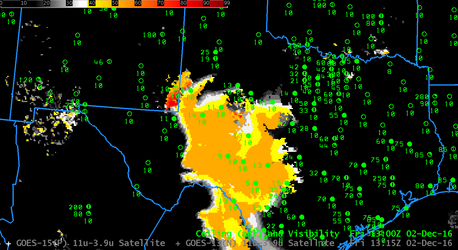
It is possible to alter the Brightness Temperature Difference Colormap, as below (animation courtesy Mike Stavish, SOO at Medford) to better highlight regions of fog in this case.  Note in this enhancement the cirrus clouds appear white, rather than dark, as well.

GOES-15 Brightness Temperature Difference  (3.9 µm – 10.7 µm) Fields, hourly from 0800 to 1400 UTC on 21 December 2016 (Click to enlarge)

The toggle below shows two color enhancements at 1200 UTC: the default version with many orange pixels, and an altered version that shows fewer pixels, mostly in regions where fog is present. A similar toggle for 0400 UTC is here.

Brightness Temperature Difference (3.9 µm – 10.7 µm) fields at 1200 UTC with two different enhancements. (Click to enlarge)

IFR Conditions across the Deep South

GOES-R IFR Probability computed with GOES-13 and Rapid Refresh Model Data, hourly from 0215 through 1415 UTC on 20 December 2016 (Click to enlarge)

Widespread IFR Conditions developed across Mississippi, Alabama, Georgia and neighboring states on Tuesday morning 20 December, as evidenced by the Aviation Weather Center website screen grab at the bottom. GOES-R IFR Probabilities captured the evolution of the low ceilings and reduced visibilities. In particular, note in the animation above the westward progress of the higher IFR probabilities through Mississippi; IFR conditions develop at, for example, Jackson (KJAN), Greenwood (KGWO) and Oxford (KUOX) as the high probabilities move over the station. Its motion was useful as a forecast tool on this morning.

The GOES-R IFR Probability field has noticeable stripes in it at the end of the animation.  This occurs because high clouds have overspread the low stratus/fog.  When that happens, satellite data can no longer be used as a predictor in the IFR Probability algorithm because the satellite can no longer view the low clouds;  Rapid Refresh data alone are driving the values.  The toggle between the brightness temperature difference field (3.9 µm – 10.7 µm) and the IFR Probability field, below, from 1115 UTC on 20 December, shows the effect.  Where fog/stratus are present (yellow in the enhancement used for the brightness temperature difference field), IFR Probability values are larger because satellite and model data can be used to compute IFR Probability.  Where high clouds are present (dark grey in the brightness temperature difference enhancement), only Rapid Refresh data can be used.

GOES-R IFR Probability and GOES-13 Brightness Temperature Difference (3.9 µm – 10.7 µm) fields, 1115 UTC on 20 December 2016 (Click to enlarge)

Aviation Weather Center website screengrab, 1443 UTC on 20 December 2016 (Click to enlarge)

Fog over South Texas

Toggle between Brightness Temperature Difference (3.9µm – 10.7µm) and GOES-R IFR Probability fields, 2300 UTC on 11 December 2016 (Click to enlarge)

Dense Fog developed over south Texas during the early morning of 12 December 2016 (IFR Sigmet from this website shown here ; Advisories from the weather.gov website shown here). The toggle above shows in the brightness temperature difference field a signature of high clouds — and where those high clouds exist, IFR Probability fields rely on Rapid Refresh Model data to diagnose where IFR conditions might be occurring, or where IFR conditions might develop. The animation of Brightness Temperature Difference fields from 0215 through 1115 UTC, below, shows that the high clouds over south Texas diminished with time: by 0815 UTC only low stratus is present over south Texas.  But is that stratus also hugging the ground — that is, is it fog?  From the satellite’s perspective, the top of a stratus deck and the top of a fog bank can look very similar.

GOES-13 Brightness Temperature Difference (3.9µm – 10.7µm), 0215 through 1115 UTC on 12 December (Click to enlarge)

GOES-R IFR Probability fields give a more complete estimate about the presence of fog/low stratus because Rapid Refresh data and satellite data are used to diagnose the probability of IFR conditions. If the Rapid Refresh model shows low-level saturation, then the presence of stratus clouds also likely indicates the presence of fog; conversely, if the Rapid Refresh Model does not show low-level saturation, then the presence of stratus cloud need not indicate the presence of fog. IFR Probability fields below, from 0215 through 1115 UTC, start off regions with uniform values where only Rapid Refresh data are used in the algorithm — where high clouds block the satellite view of low clouds/fog. As the high clouds dissipate, the field acquires larger values because there is higher confidence of the presence of clouds (in part because satellite data can be used to observe them). In addition, these larger values have pixel-sized variability because of variability in the satellite observations.

IFR conditions are observed latest over far south Texas — this is also where IFR Probabilities are slowest to reach large values.

Fog and Ice Fog over the southern Plains

ifrp_0400_1215_05dec2016anim

GOES-R IFR Probabilities, hourly from 0400 through 1215 UTC on 5 December 2016 (Click to enlarge)

Dense Fog developed over the southern Plains early on Monday 5 December, and the GOES-R IFR Probability fields, above, were a tool that could be used to monitor the evolution of this event. A challenge presented on this date was the widespread cirrus (Here’s the 0700 UTC GOES-13 Water Vapor (6.5 µm) Image, for example) that prevented satellite detection of low clouds. The Brightness Temperature Difference fields, below, at 3-hourly intervals, also show a signature (dark grey/black in the enhancement used) of high clouds, although they are shifting east with time — by 1300 UTC there is a signature (orange/yellow in the enhancement used) of stratus clouds over central and eastern Oklahoma.

The IFR Probability fields, above, have a characteristic flat nature over Arkansas and Missouri, that is, a uniformity to the field, that is typical when model data are driving the probabilities. The more pixelated nature to the fields over Kansas and Oklahoma, especially near the end of the animation, typifies what the fields look like when both satellite data and model data are driving the computation of probabilities. Careful inspection of the fields over Arkansas shows regions — around Fayetteville, for example, around 1000 UTC where IFR Probabilities are too low given the observation at the airport of IFR conditions. This inconsistency gives information on either the small-scale nature of the fog (unlikely in this case) or on the accuracy of the Rapid Refresh model simulation that is contributing to the probabilities. In general, the Rapid Refresh model has accurately captured this event, and therefore the IFR Probabilities are mostly overlapping regions of IFR or near-IFR conditions. The region over southern Illinois that has stratus, and low probabilities of IFR conditions, for example. Adjacent regions have higher IFR Probabilities and lower ceilings and/or reduced visibilities. A screen shot from the National Weather Service, and from the Aviation Weather Center, at about 1300 UTC document the advisories that were issued for this event.

btd_0400_1300_05dec2016step

Brightness Temperature Difference fields (3.9 µm – 10.7 µm), 0400, 0700, 1000 and 1300 UTC on 5 December 2016 (Click to enlarge)

IFR Conditions over the High Plains of west Texas

goes_btd_ifr_0215_1415_02dec2016anim

GOES-13 Brightness Temperature Difference (3.9 µm – 10.7 µm, left) and GOES-R IFR Probability Fields (Right), hourly from 0215 through 1415 UTC on 2 December 2016 (Click to enlarge)

Near-IFR and and IFR Conditions developed over the High Plains of Texas on 2 December 2016, and a SIGMET for IFR conditions was issued as shown below.

The animation above shows plentiful cirrus (in the brightness temperature difference enhancement used in the imagery on the left, above, cirrus clouds are dark) over south Texas, with occasional breaks.  This makes continual monitoring via satellite of the developing stratus/fog field problematic:  the satellite cannot monitor what it is blocked from being observed by intervening cloud layers — in this case cirrus.  (Click here for a brightness temperature difference only animationClick here for an IFR Probability only animation)  Because IFR Probability fields include model-based data about saturation in the lower troposphere, in the form of Rapid Refresh model output, a useful and coherent signal can be generated underneath cirrus clouds.  The GOES-R IFR Probability signal can be better used for situational awareness and anticipation of the development of the IFR conditions shown below.

In the animation above, note the change between 1315 and 1415 UTC fields — in the Brightness Temperature Difference fields (1315 UTC ; 1415 UTC), this change arises because of increasing amounts of reflected solar 3.9 µm radiation:  this causes a sign change in the brightness temperature difference.  For IFR Probability fields (1315 UTC ; 1415 UTC), the change occurs because the Predictors used at night (1315 UTC) and during the day (1415 UTC) are different.

awc_1600utc_2december2016

1605 UTC screen capture from Aviation Weather Center. Note IFR Sigmet over west Texas (Click to enlarge)