Monthly Archives: October 2015

Benefit of fused data over Oklahoma

GOES-R IFR Probabilities (Upper Left), GOES-R Cloud Thickness (Lower Left), GOES-13 Brightness Temperature Difference (10.7 µm – 3.9 µm) (Upper Right), GOES-13 Water Vapor Infrared Imagery (6.5 µm) (Lower Right), all at 1100 UTC on 28 October 2015 (Click to enlarge)

Fused Data is beneficial in the detection of low ceilings and reduced visibilities. Consider the region in northeastern Oklahoma where cirrus has overspread low clouds and dense fog is reported on the ground. The satellite view of the low clouds is obscured by the cirrus; the brightness temperature difference signal is not one associated with fog/low stratus. However, GOES-R IFR Probability fields maintain a signal because Rapid Refresh model output is used; saturation is occurring in the lowest 1000 feet of the model over eastern OK, and the GOES-R IFR Probability is larger there as a result. (Dense Fog Advisories were issued for this event).

Dense Fog Detection over western North Dakota under Cirrus

Dense fog formed over western North Dakota early in the morning of Monday 26 October (and advisories were issued). At the same time, cirrus clouds overspread the region, making satellite detection of the low clouds problematic. This is an excellent example of the benefits of a fused product that blends surface and near-surface information from numerical models with satellite detection. When one of the products gives no information, the other can be relied upon to fill in gaps.

In the example above, dense fog develops over western North Dakota, complete with freezing drizzle. Satellite detection of the low clouds on this date was difficult because of widespread cirrus that overspread the state; these cirrus are apparent in both the water vapor (lower right) and the brightness temperature difference (upper right). When model data principally are used to compute the IFR Probability fields — in regions where high clouds prevent a satellite view of low clouds — the character of the field is flatter and less pixelated. In addition, where high clouds cannot view low clouds, the Cloud Thickness cannot be computed (as it relates 3.9µm emissivity to cloud thickness). Note that there are regions where the cirrus thins enough that low clouds can be viewed — in these regions the Cloud Thickness is computed an the IFR Probability increases (where both Cloud Predictors and Model Predictors can be used, IFR Probabilities are larger).

Fog in the Carolinas

GOES-R IFR Probabilities, hourly from 0000 UTC through 1315 UTC on 22 October 2015 (Click to enlarge)

Dense fog developed over South and North Carolina on the morning of 22 October 2015, just inland from the coast (Click here for screenshot from the National Weather Service homepage from Wilmington NC). The animation, above, shows the hourly evolution of the GOES-R IFR Probability fields from just after sunset on the 21st through sunrise on the 22nd. Highest probabilities of IFR Conditions overlap the stations where IFR Conditions occur. GOES-R Cloud Thickness also gives information on where the thickest clouds are; the 1115 UTC Cloud Thickness (the final field before twilight conditions change the 3.9 µm emissivity used to diagnose Cloud Thickness) shows the thickest clouds removed from the coast; compare that region to the regions with fog remaining at 1315 UTC in the animation above. There is good overlap. The maximum cloud thickness in the just-before-sunrise image below is a bit over 1000 feet, in northeastern North Carolina; according to this scatterplot that relates pre-sunrise cloud thickness to dissipation time, fog dissipation should occur within 3 hours, that is by 1415 UTC.

GOES-R Cloud Thickness, 1115 UTC on 22 October (Click to enlarge)

IFR Probabilities have better statistics in outlining regions of dense fog. This is because fog that reduces visibility and low stratus that does not reduce visibility can look very similar to a satellite. IFR Probability fields incorporate near-surface information in the guise of Rapid Refresh model predictions of low-level saturation that better refine regions where low stratus extends down to the ground. There are regions where brightness temperature difference has a fog-like signal with high ceilings/good visibility (central South Carolina, for example). These regions have low IFR Probability values because the Rapid Refresh model does not predict low-level saturation. Fusing satellite and model data yields a better product.

GOES-13 Brightness Temperature Difference (10.7µm – 3.9µm) and IFR Probability fields, 0615 UTC on 22 October 2015 (Click to enlarge)

The visible animation, below, shows that fog dissipated completely shortly after 1430 UTC, in accordance with expectations based on the Cloud Thickness.

GOES-13 Visible Imagery, 1315 through 1445 UTC on 22 October (Click to enlarge)

Resolution Benefits from MODIS

GOES-R IFR Probability fields, every 2 hours from 0200 through 1400 UTC on 16 October 2015 (Click to enlarge)

The GOES-R IFR Probability fields over Oregon and Washington on the morning of 16 October 2015 correctly diagnose low ceilings and reduced visibilities along the coast, even when high clouds intervene at the end of the animation above (especially evident at 1300 UTC, below). In addition to marine stratus that is reducing visibility/ceilings along the coast, surface observations suggest a valley fog is forming in/around Centralia/Chehalis Washington (KCLS). However, GOES-based IFR Probability fields do not become enhanced in that area. Why not?

GOES-R IFR Probability computed from GOES-15, 1300 UTC on 16 October 2015. Note the Character of the field near Newport OR (KONP); the uniformity of the field is characteristic of regions where satellite signals cannot be used because of high clouds (Click to enlarge)

The valley of the Chehalis River, in which the fog is forming, is far too narrow to be resolved by GOES-15, which satellite has 4-km pixel sizes at the sub-satellite point. (Pixels are closer to 6 km in size over southern Washington). Higher-resolution MODIS data (with a 1-km pixel size) can be used to create GOES-R IFR Probabilities, and MODIS overpasses viewed Centralia/Chehalis at 0650, 0924 and 1105 UTC. The imagery below toggles between MODIS-based and GOES-based GOES-R IFR Probabilities at those times. Even as early as 0645 UTC, the MODIS-based IFR Probability fields are suggesting that a fog is starting to develop. At later times the MODIS-based IFR Probability values are much larger than the GOES-based values. MODIS data can give an early alert to the development of small-scale fog.

MODIS-based (0650 UTC) and GOES-15-based (0645 UTC) GOES-R IFR Probability fields (Click to enlarge)

MODIS-based (0924 UTC) and GOES-15-based (0930 UTC) GOES-R IFR Probability fields (Click to enlarge)

MODIS-based (1105 UTC) and GOES-15-based (1100 UTC) GOES-R IFR Probability fields (Click to enlarge)

Fog over South Georgia

GOES-R IFR Probability fields (Upper left), GOES-13 Brightness Temperature Difference (10.7 µm – 3.9 µm) Fields (Upper Right), GOES-R Cloud Thickness (Lower Left), GOES-13 Infrared Water Vapor (6.5 µm) Imagery (Lower Right), all at 1115 UTC 9 October 2015

Dense fog formed over south Georgia early in the morning of 9 October 2015 (National Weather Service Homepage in Peachtree City). The imagery above, from 1115 UTC, demonstrates a strength of the GOES-R IFR Probability field: it maintains a signal where dense fog is ongoing even as high clouds overspread the region. At 0800 UTC on 9 October (below), high clouds had not yet overspread south Georgia, and the image below shows that both IFR Probabilities and Brightness Temperatuere Difference fields outline the region of developing fog. When high clouds appear (as in the image above), the Brightness Temperature Difference signal that can be used in clear skies loses its utility in fog detection.

As above, but at 0800 UTC 9 October 2015

IFR Probability discriminates between Low Stratus and Mid-Level Stratus

Dense Fog Advisories were issued over parts of eastern North Dakota (Screenshot of Grand Forks National Weather Service Page) early on 9 October:

URGENT – WEATHER MESSAGE
NATIONAL WEATHER SERVICE GRAND FORKS ND
303 AM CDT FRI OCT 9 2015

NDZ006-007-014-015-024-028-038-091500-
/O.NEW.KFGF.FG.Y.0006.151009T0803Z-151009T1500Z/
/O.CON.KFGF.FR.Y.0011.000000T0000Z-151009T1400Z/
TOWNER-CAVALIER-BENSON-RAMSEY-EDDY-GRIGGS-BARNES-
INCLUDING THE CITIES OF…CANDO…LANGDON…FORT TOTTEN…
MADDOCK…LEEDS…MINNEWAUKAN…DEVILS LAKE…NEW ROCKFORD…
COOPERSTOWN…VALLEY CITY
303 AM CDT FRI OCT 9 2015

…DENSE FOG ADVISORY IN EFFECT UNTIL 10 AM CDT THIS MORNING…
…FROST ADVISORY REMAINS IN EFFECT UNTIL 9 AM CDT THIS MORNING…

THE NATIONAL WEATHER SERVICE IN GRAND FORKS HAS ISSUED A DENSE
FOG ADVISORY…WHICH IS IN EFFECT UNTIL 10 AM CDT THIS MORNING.

* TEMPERATURES…IN THE LOWER 30S.

* VISIBILITIES…AREAS OF VISIBILITY UNDER ONE QUARTER MILE.
VISIBILITIES WILL BE HIGHLY VARIABLE HOWEVER.

* TIMING…FOG WILL BURN OFF MID MORNING.

PRECAUTIONARY/PREPAREDNESS ACTIONS…

A FROST ADVISORY MEANS THAT WIDESPREAD FROST IS EXPECTED.
SENSITIVE OUTDOOR PLANTS MAY BE KILLED IF LEFT UNCOVERED.

A DENSE FOG ADVISORY MEANS VISIBILITIES WILL FREQUENTLY BE
REDUCED TO LESS THAN ONE QUARTER MILE. IF DRIVING…SLOW DOWN…
USE YOUR HEADLIGHTS…AND LEAVE PLENTY OF DISTANCE AHEAD OF YOU.

GOESR_IFRPROB_0200_1100_09October2015anim

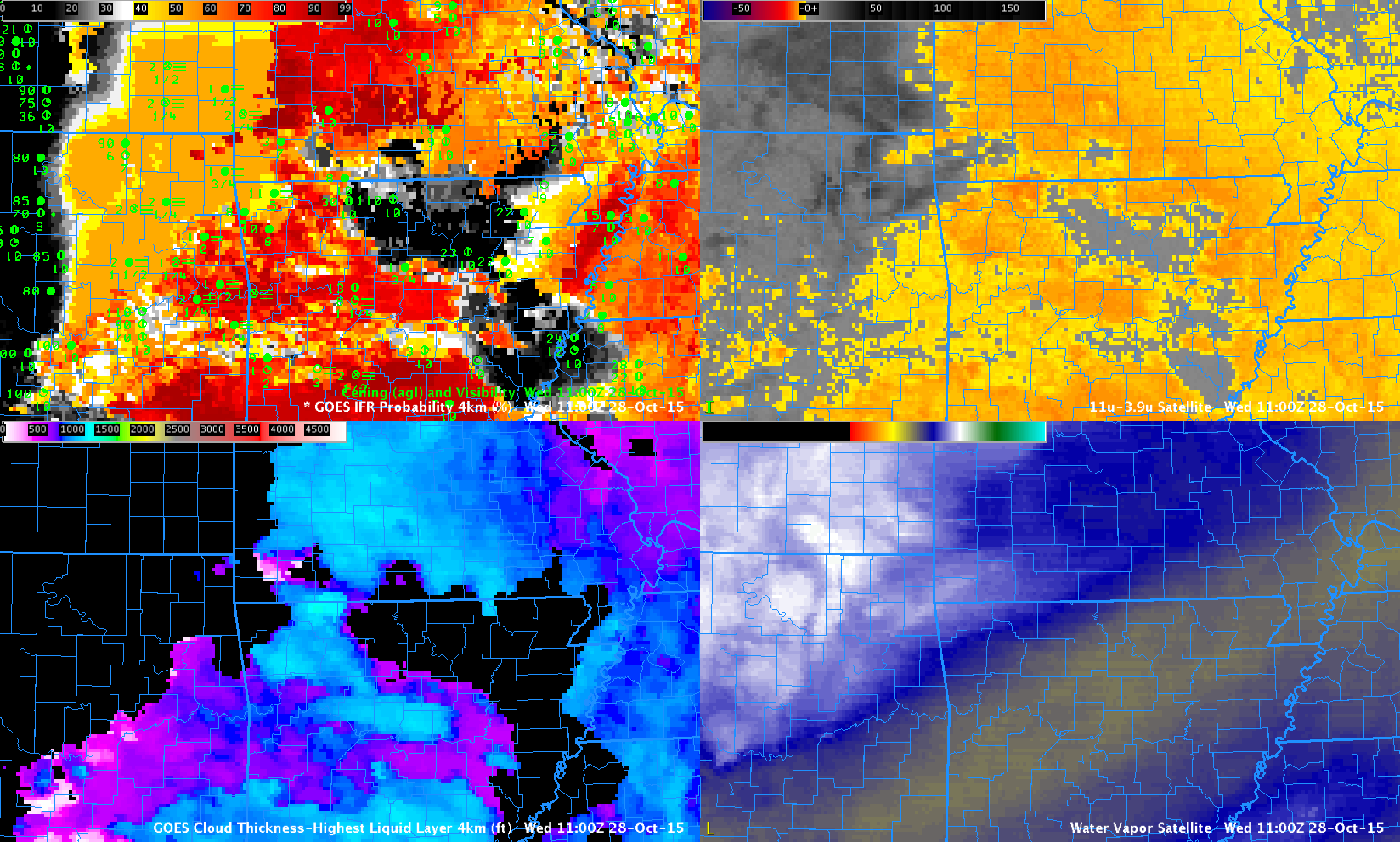
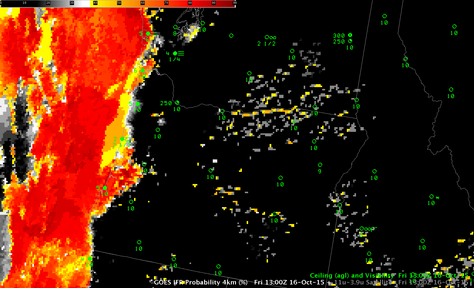
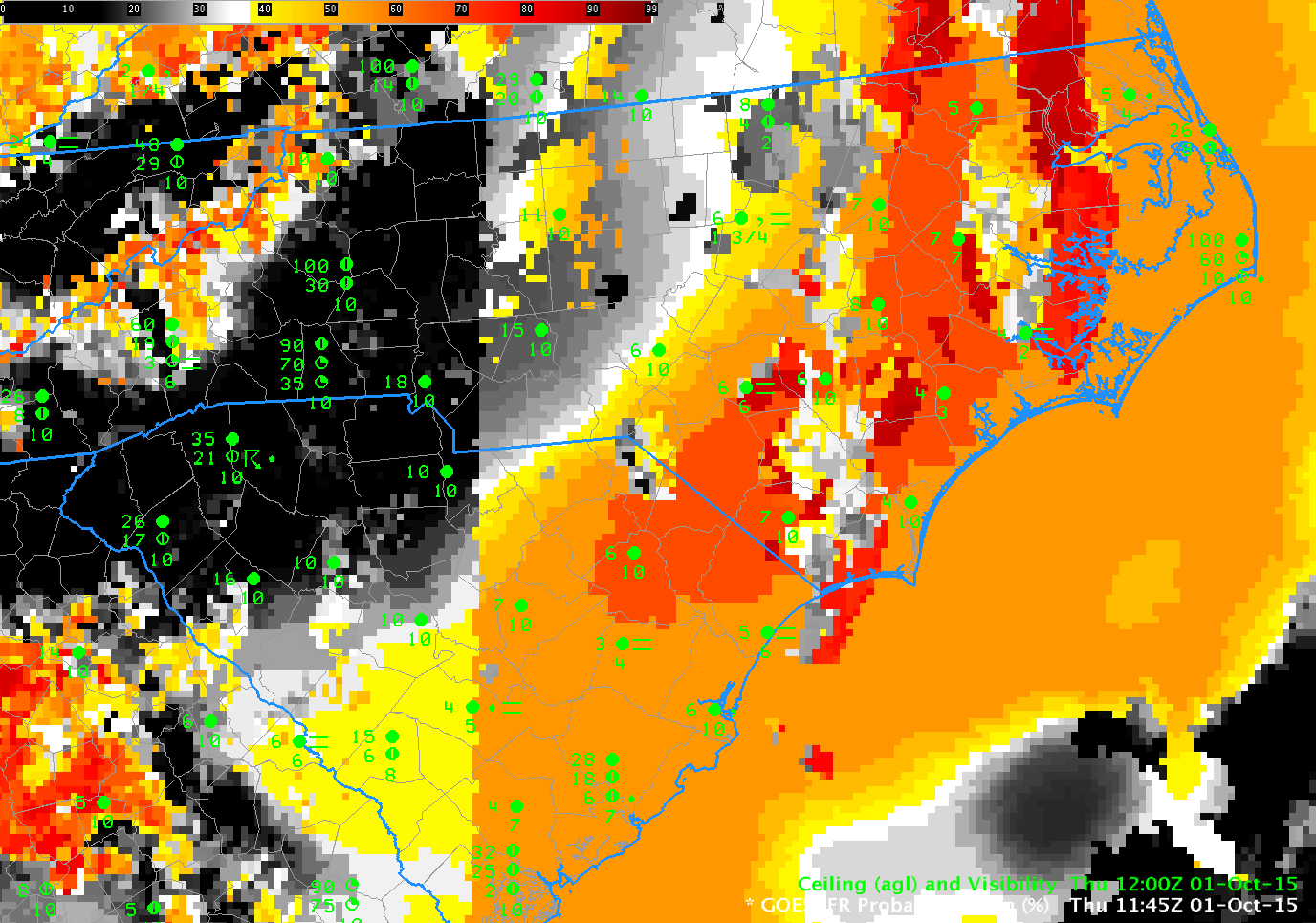
GOES-R IFR Probability Fields and surface reports of ceilings and visibilities, 0200-1100 UTC (Click to enlarge)

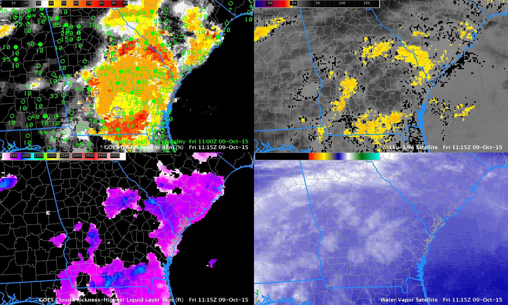
The GOES-R IFR Probability fields increased in this region as the fog developed (above). Notably in this case, IFR probabilities were lower over Minnesota and the Red River Valley where mid-level stratus was occurring. The toggle below compares IFR Probabilities and Brightness Temperature Differences at four times during the night. The Brightness Temperature Difference fields (animation from 0400-1100 UTC is here) greatly overpredict the region of dense fog. Because the IFR Probabilities incorporate information about the surface, however, regions of mid-level stratus can be screened out. These are regions where the Rapid Refresh model does not show saturation in the lowest layers.

Note that Cirrus is overspreading the region from the west at the end of the animations. High Clouds change the signal in the brightness temperature difference field. Harvey ND at 1100 UTC reports Zero visibility and an obscured ceiling (with freezing drizzle). The station is under cirrus, however, so a brightness temperature difference signal associated with fog is not present. There is a modest IFR Probability value there because data from the Rapid Refresh suggests low-level saturation is occurring.

GOESR_BTD_IFRPROB_4_6_8_1100_09October2015toggle_4PANEL

GOES-13 Brightness Temperature Difference fields and GOES-R IFR Probability Fields at 0400 (Upper Left), 0615 (Upper Right), 0800 (Lower Left) and 1100 (Lower Right) [Click to enlarge]

Fog under high clouds in Indiana

GOES-R IFR Probability (Upper Left), GOES-R Low IFR Probability (Lower Left), GOES-13 Brightness Temperature Difference (10.7µm – 3.9µm) (Upper Right), GOES-R Cloud Thickness (Lower Right) (Click to enlarge)

Fog developed over Indiana and surrouding states (again) on the morning of 6 October, and the animation above traces that development as diagnosed by GOES-R IFR Probability fields. Multiple cloud layers over the region meant that the Brightness Temperature Difference field, a traditional method of low cloud detection (that keys on the differences in emissivity at 10.7 and 3.9 in water-based clouds) could not be used because low cloud detection was hampered by the presence of high clouds. The fused product, GOES-R IFR Probability, provides useful information by combining Rapid Refresh Data information about low-level saturation with satellite fields. When satellite information about low clouds are missing, as in this case, model data provides a signal.

Because multiple cloud layers exist, the GOES-R Cloud Thickness Product (that diagnoses the depth of the lowest water-based cloud based on an empirical relationship between 3.9 µm emissivity and cloud depth developed using sodar observations off the West Coast of the United States) is not produced over much of the region. It is also not produced at times of twilight — such as those that occur at the end of the animation. There are values over southeastern lower Michigan at the start of the animation, where high clouds were not present.

Low IFR Probability is also shown in the animation above (Lower Left figures). The small values in this case suggest any fog is unlikely to be producing visibilities less than 1 mile or ceilings less than 500 feet.

IFR Probabilities when thick clouds are present

Suomi NPP Day Night Visible (0.70 µm) Image, 0744 UTC on 1 October 2015 (Click to enlarge)

When thick clouds are present, as along the East Coast of the United States early on 1 October 2015, as depicted by the Suomi NPP Day Night band (0.70 µm) image above, satellite detection of low clouds is problematic. This is why GOES-R IFR Probability fields incorporate information from model data so that useful guidance can be produced on whether IFR Conditions exist.

IFR Probabilities increase slowly over coastal South and North Carolina after midnight on 1 October — and the fields do a good job of outlining where IFR Conditions are occurring. In most locations, at most times, the fields are not pixelated. The smooth nature arises when model fields (which are relatively smooth) are used (and satellite data that are more pixelated are not used) to generate the IFR Probability Fields. Some holes in the extensive cloud cover occur over North Carolina during the animation: the IFR Probability field takes on a more pixelated appearance when that happens — and the Probability value increases when satellite data can also be used as a Predictor.

GOES-R IFR Probability fields created with GOES-13 Imager and Rapid Refresh model Data, 0500-1215 UTC on 1 October 2015 (Click to enlarge)

The GOES-R IFR Probability field at 1145 UTC includes a north-south oriented artifact. To the east of the obvious line, day-time predictors are used in the GOES-R IFR Probability computation; to the west, night-time predictors are used. One of the daytime predictors is Visible Imagery that is used to cloud-clear more accurately. The IFR Probability where daytime predictors are used is larger because there is more confidence that a cloud does exist.

GOES-R Fog Product Examples

Fog detection fusing GOES, Terra/Aqua or Suomi/NPP Satellite data with Model output