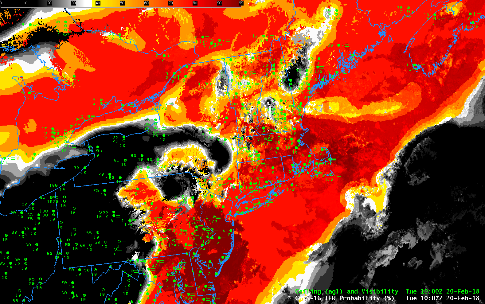
GOES-16 IFR Probability, 1007 UTC on 20 February 2018, along with surface observations of ceilings and visibilities (Click to enlarge)
A complex set of Low Pressure systems over the eastern half of the United States brought multiple cloud layers and IFR conditions to the northeastern United States on 20 February. The image above shows the IFR Probability field at 1007 UTC. IFR Conditions are apparent from the Chesapeake Bay northeastward through southeastern Pennsylvania and New York and coastal New England, as well as over southeastern Ontario Province in Canada and the Canadian Maritimes. These are also regions where IFR Probabilities are high, generally exceeding 80%. In regions where IFR conditions are not observed (Western Pennsylvania and Ohio, for example), IFR Probabilities are generally small.
When multiple cloud decks are present, as occurred on 20 February, satellite-only detection of low clouds is a challenge, as shown with by the brightness temperature difference field (10.3 µm – 3.9 µm), called the ‘Night Fog’ difference in AWIPS, below. High and mid-level clouds (grey/black in the enhancement used) make satellite detection of low-level stratus impossible. So, for example, stations with IFR conditions over Long Island sit under a much different enhancement in the brightness temperature difference field compared to stations with IFR conditions over southern New Jersey and southeastern Pennsylvania.
Because the Brightness Temperature Field cannot view the low clouds, the Nighttime Microphysics RGB (shown below the Brightness Temperature Difference field) similarly cannot identify all regions of low, warm clouds — typically yellow or cyan in that RGB.
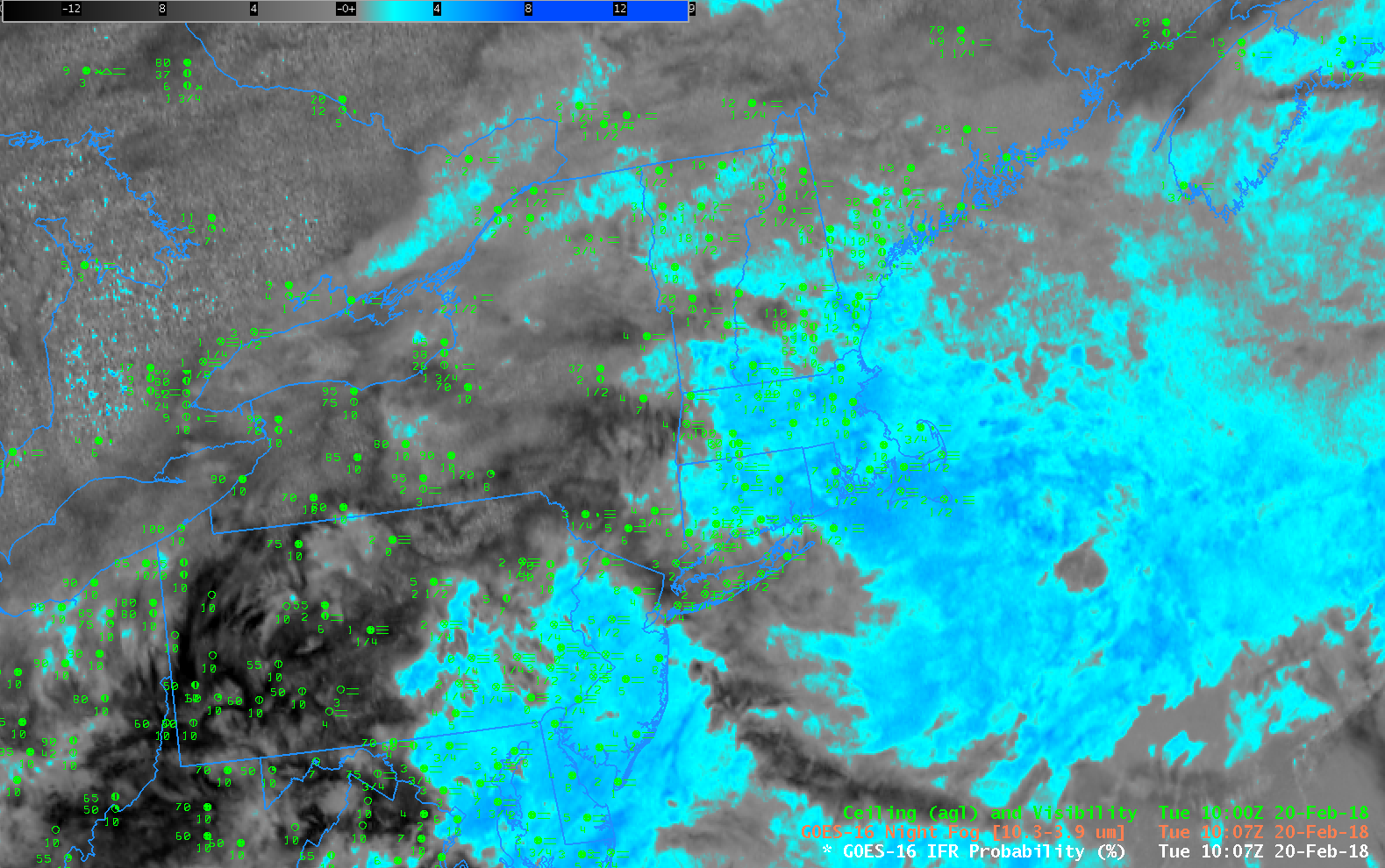
Night Fog Brightness Temperature Difference field (10.3 µm – 3.9 µm) at 1007 UTC on 20 February 2018, along with surface observations of ceilings and visibilities (Click to enlarge)
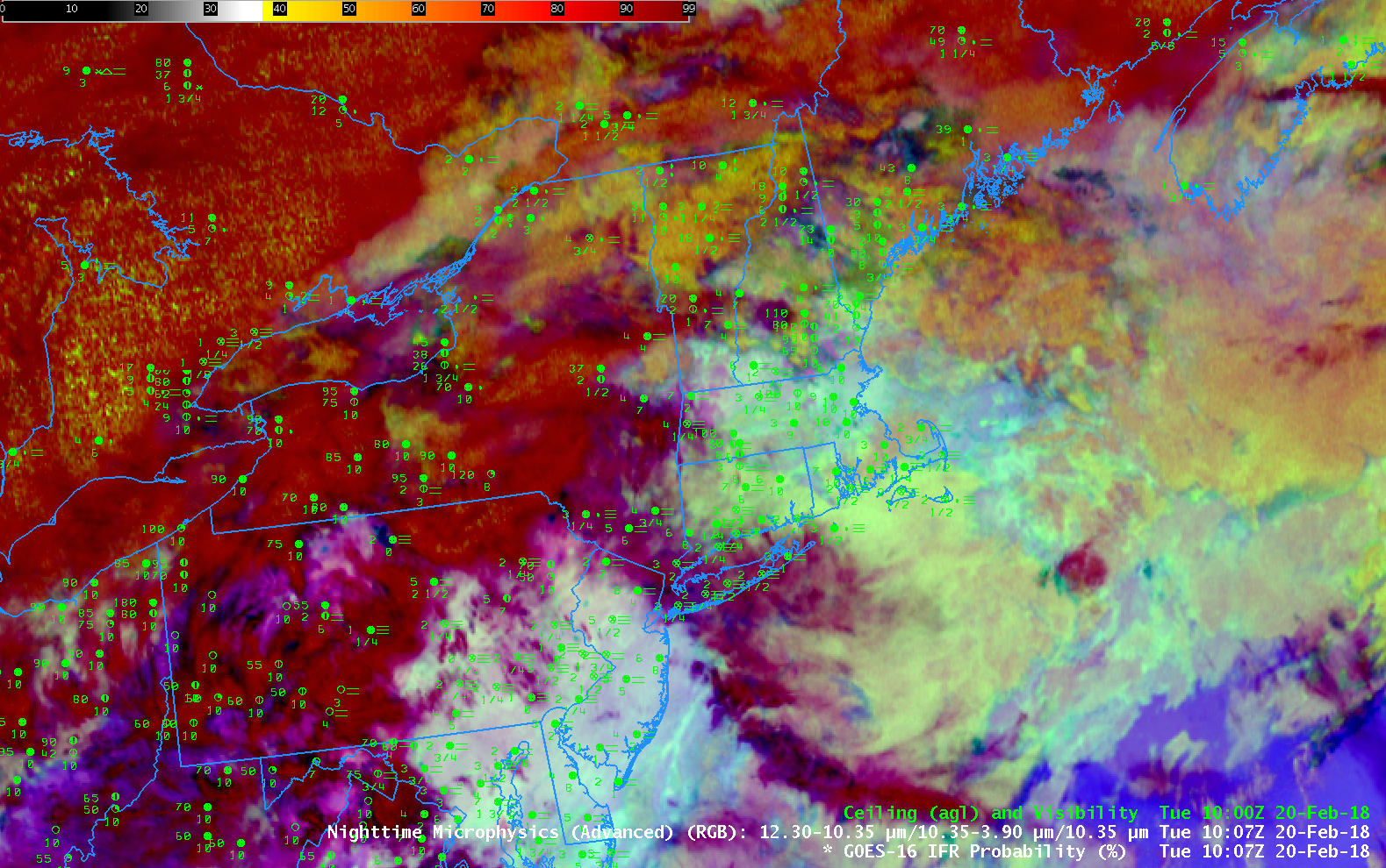
NightTime Microphysics RGB at 1007 UTC on 20 February 2018, along with surface observations of ceilings and visibilities (Click to enlarge)

