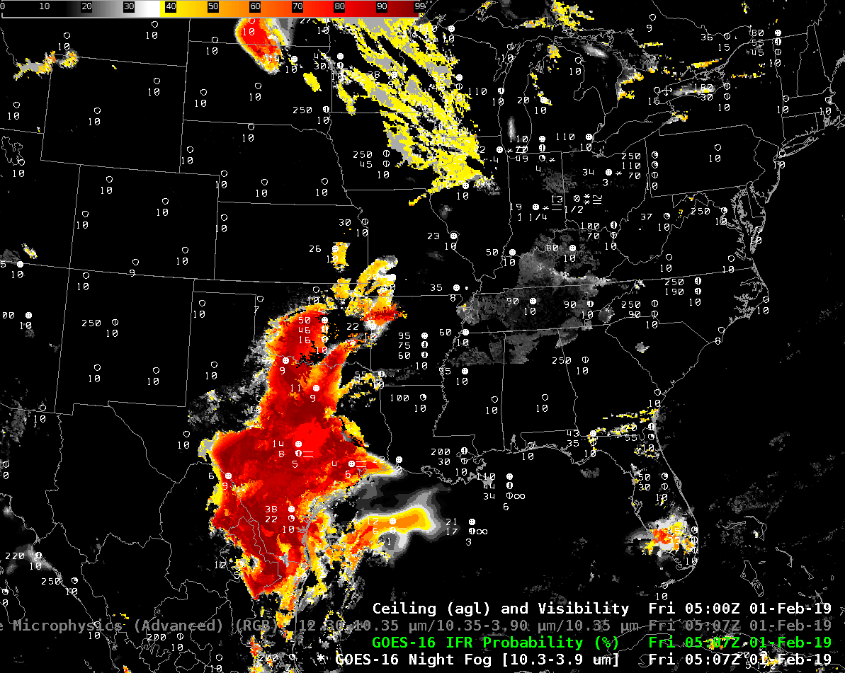
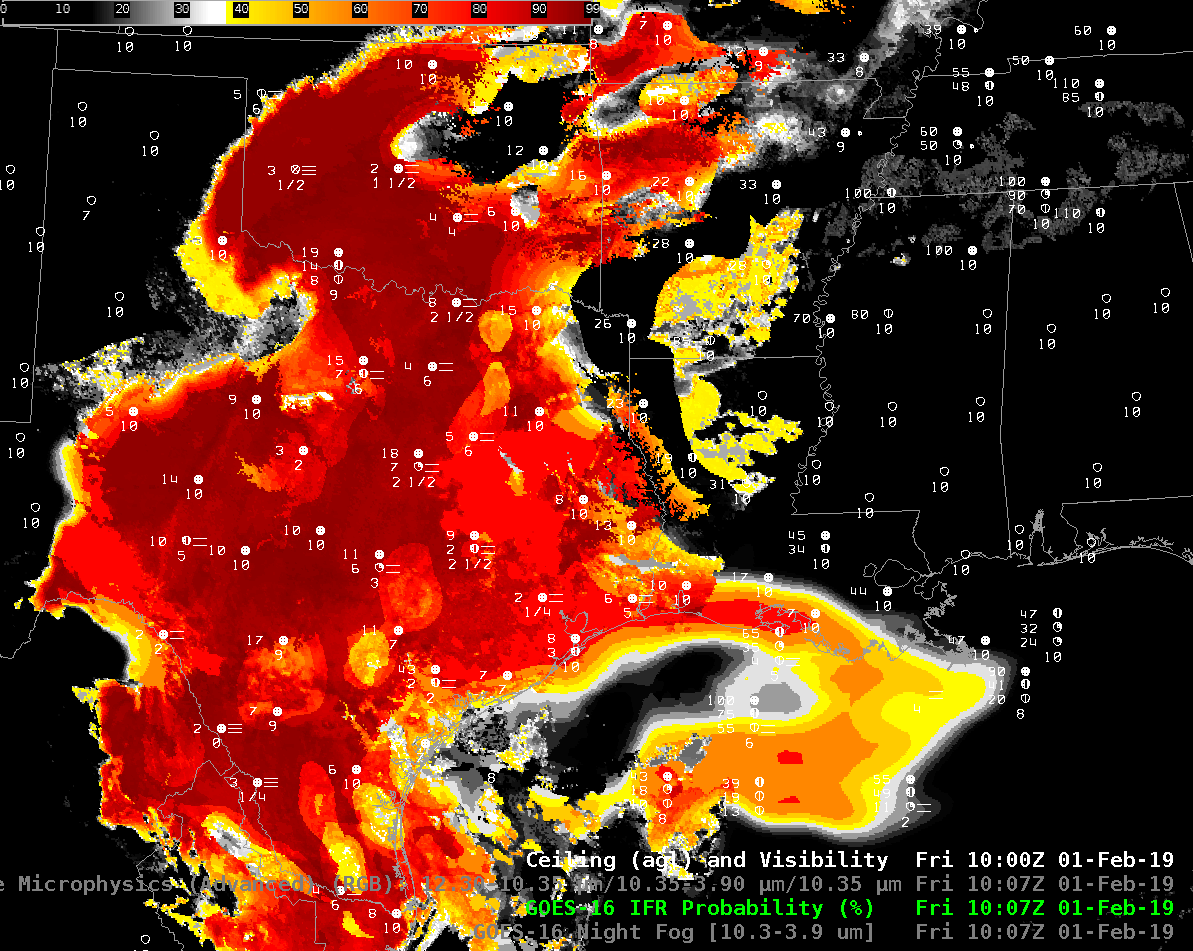
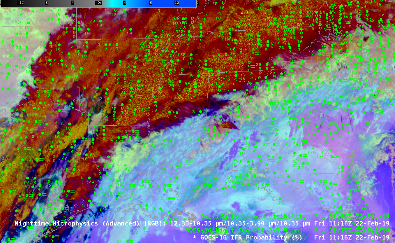
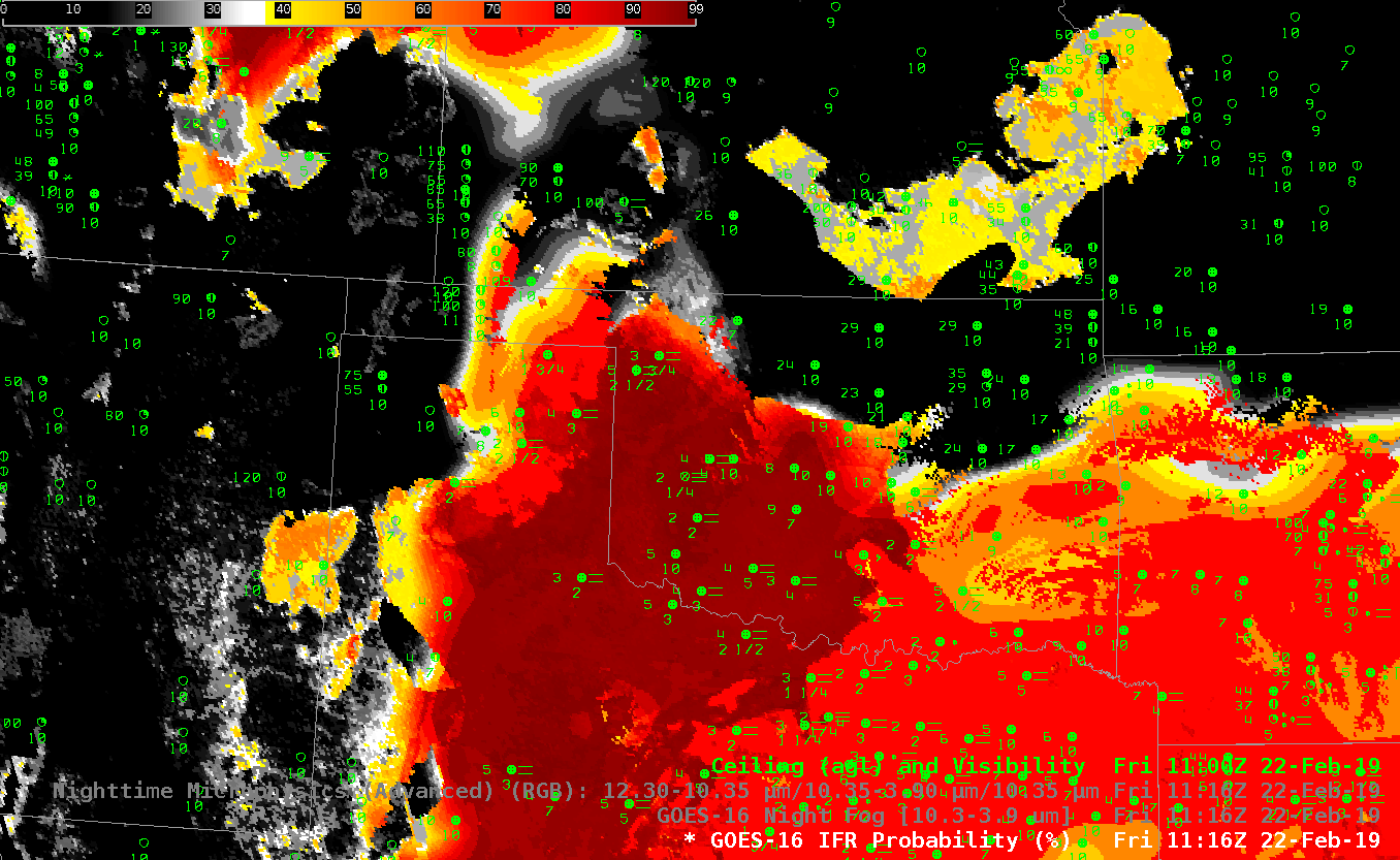
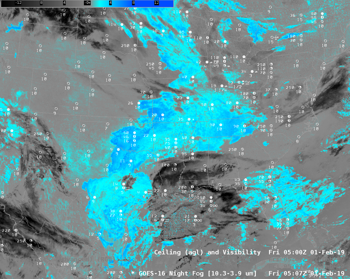
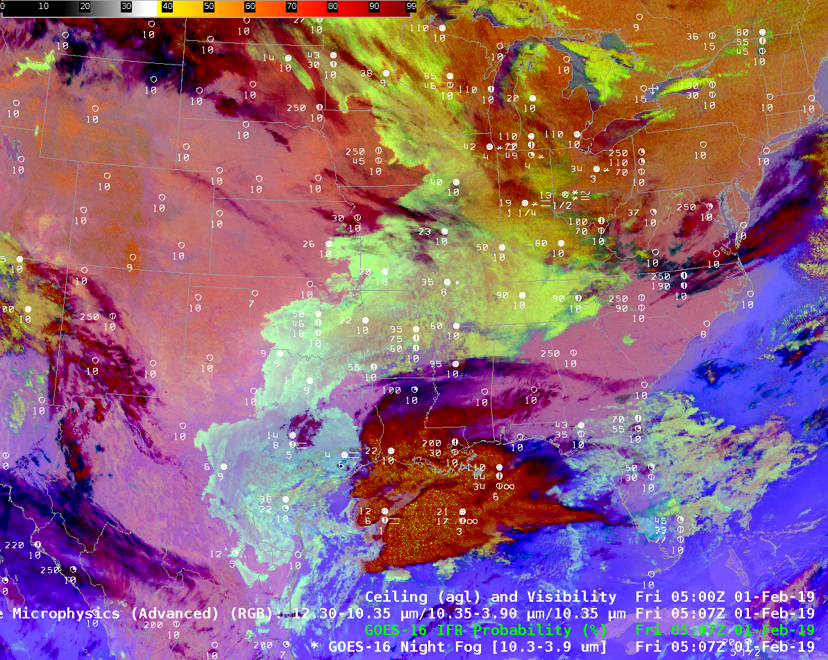
GOES-16 Night Fog Brightness Temperature Difference (10.3 µm – 3.9 µm), Nighttime Microphysics RGB and GOES-16 IFR Probability at 1116 UTC on 22 February 2019; Surface observations of ceilings and visibilities at 1100 UTC are also plotted (Click to enlarge).
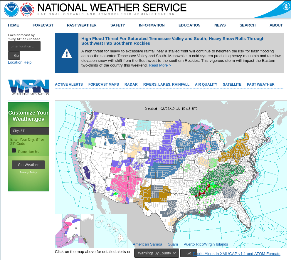
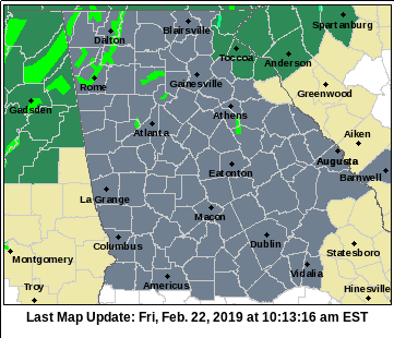
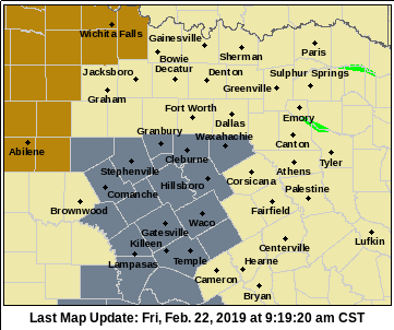
A strong storm embedded within a subtropical jet stream over the southern United States was associated with widespread fog on the morning of 22 February 2019. This screen-capture from this site shows Dense Fog Advisories over much of Georgia, and over regions near Dallas. Which products allowed an accurate depiction of the low ceilings and reduced visibilities?
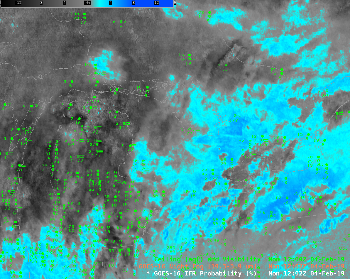
The toggle above cycles between the Night Fog Brightness Temperature Difference (10.3 µm – 3.9 µm), which product identifies low clouds (cyan blue in the default AWIPS enhancement shown) because of differences in emissivity at 3.9 µm and 10.3 µm from small water droplets that make up stratus clouds, the Nighttime Microphysics RGB, which RGB uses the Night Fog Brightness Temperature Difference as it green component, and the GOES-16 IFR Probability product. IFR conditions are defined as surface visibilities between 1 and 3 miles, and ceiling heights between 500 and 1000 feet above ground level. The plotted observations help define where that is occurring. Multiple cloud layers from Arkansas east-northeastward make a satellite-only detection of IFR conditions challenging. IFR Probability gives useful information below cloud decks because model-based saturation information from the Rapid Refresh Model fill in regions below multiple cloud decks where satellite information about low clouds is unavailable.
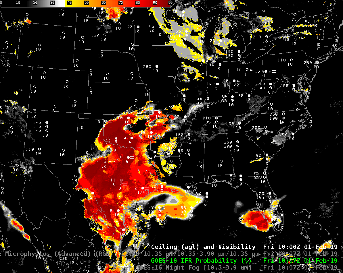
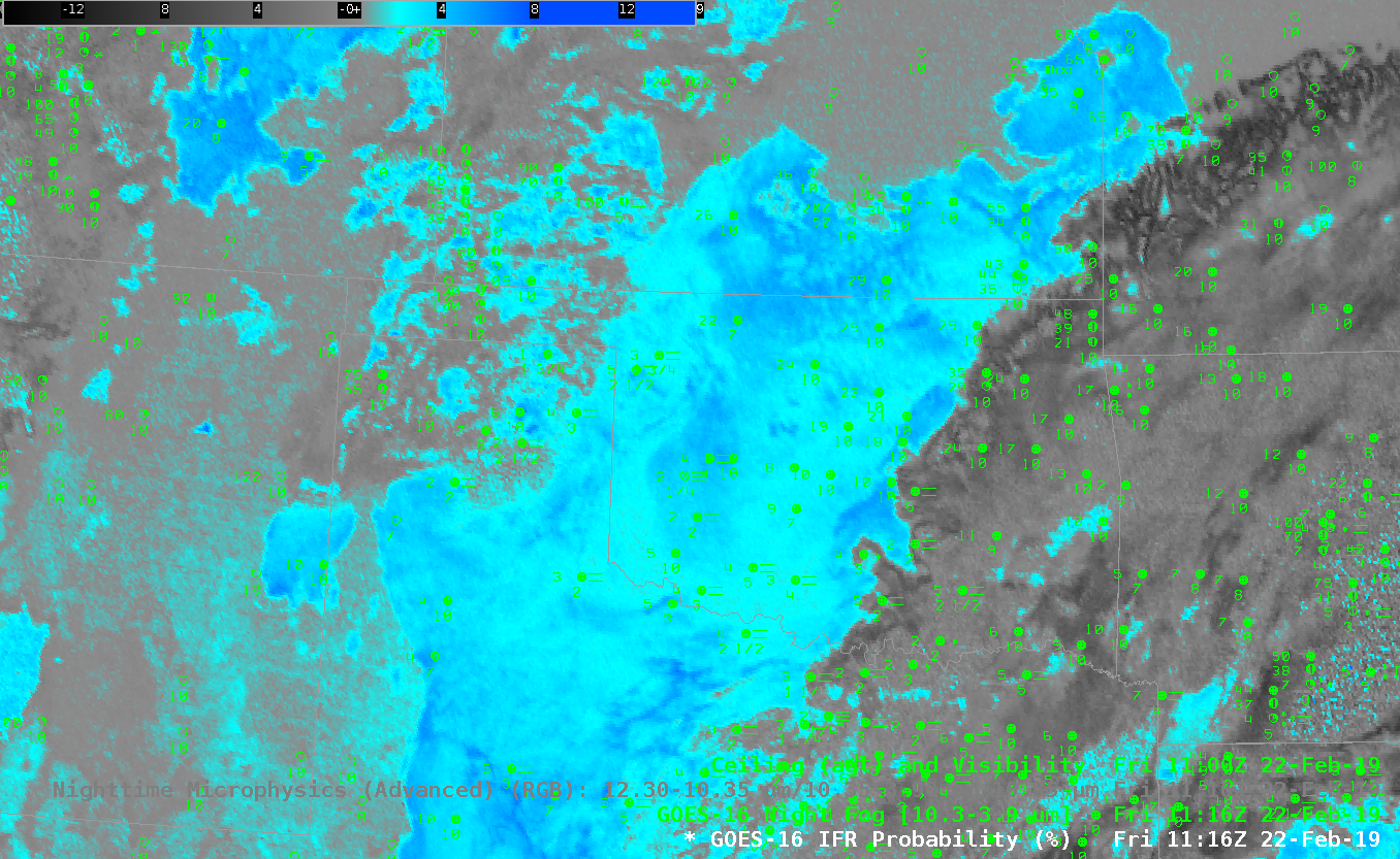
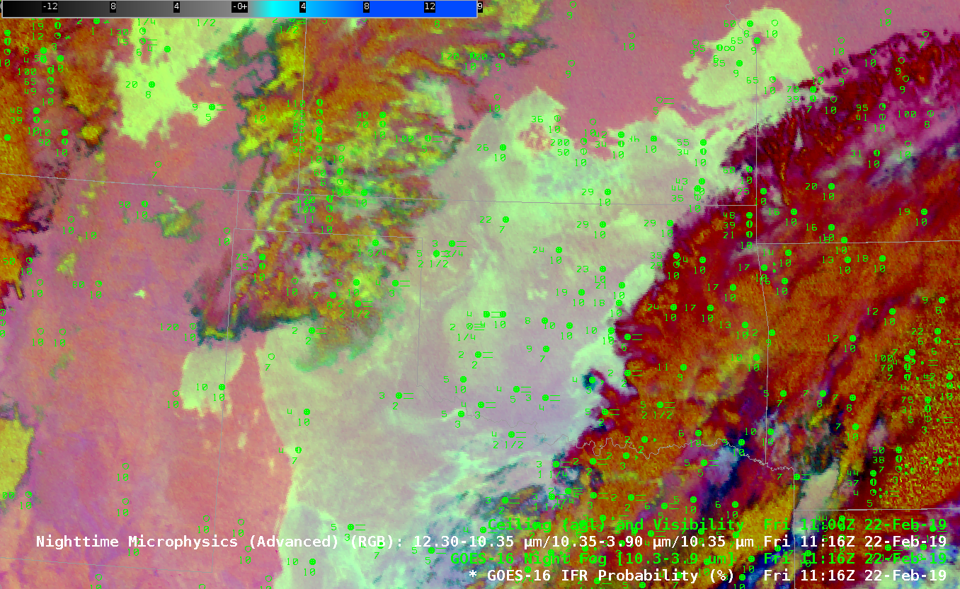
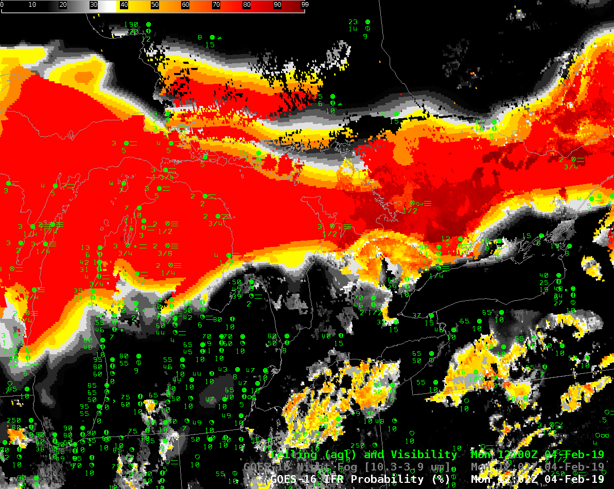
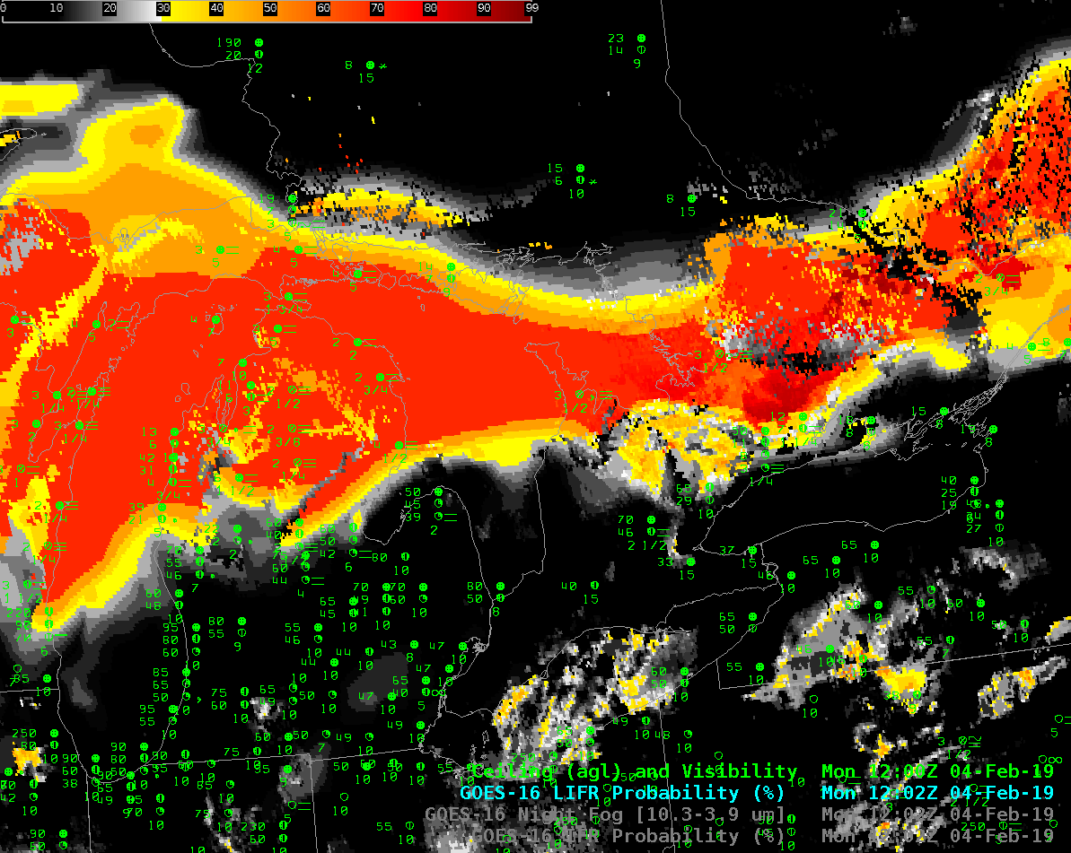
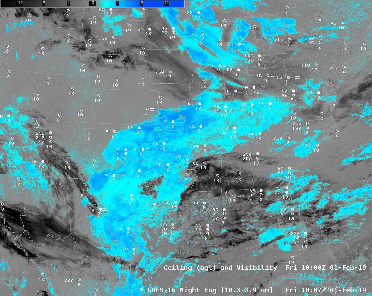
The toggle below shows the same three satellite-based fields (Night Fog Brightness Temperature Difference, Nighttime Microphysics RGB and IFR Probability) at the same time, but centered over Oklahoma. In this case, the Rapid Refresh Data are used to screen out a region of elevated stratus over northeast Oklahoma. Note that these is little in the Night Fog Brightness Temperature Difference field to distinguish between the IFR and non-IFR locations.
GOES-16 Night Fog Brightness Temperature Difference (10.3 µm – 3.9 µm), Nighttime Microphysics RGB and GOES-16 IFR Probability at 1116 UTC on 22 February 2019; Surface observations of ceilings and visibilities at 1100 UTC are also plotted (Click to enlarge).
GOES-R IFR Probability over the southeast United States in this case is identifying regions of IFR conditions underneath multiple cloud decks (and also where only the low clouds are present) by incorporating low-level saturation information from the Rapid Refresh model. Over Oklahoma, non-IFR conditions under an elevated stratus deck are identified (and screened out in IFR Probability fields) by the lack of low-level saturation information in the Rapid Refresh.


