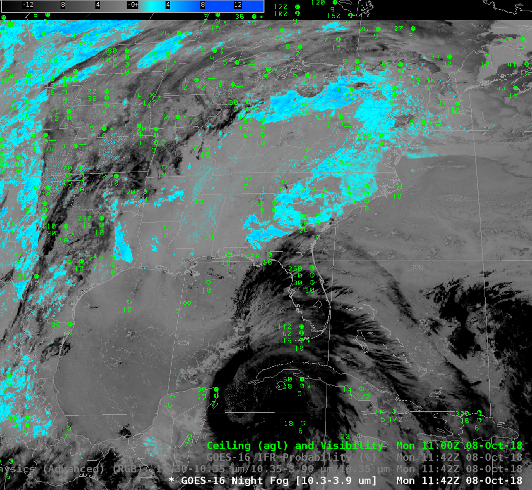
GOES-16 Night Fog Brightness Temperature Difference (10.3 µm – 3.9 µm), 1137 – 1452 UTC on 31 October 2018 (Click to animate)
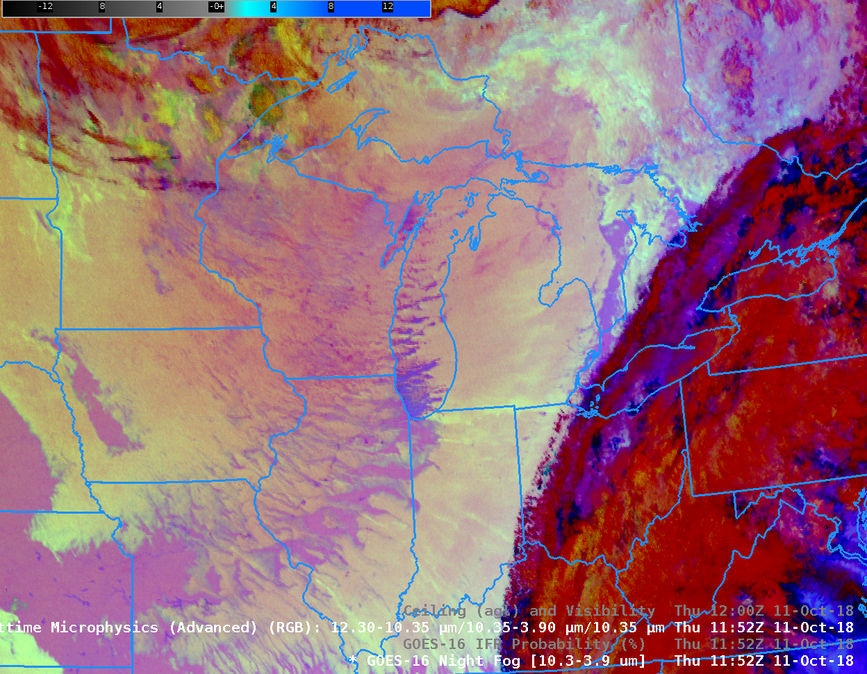
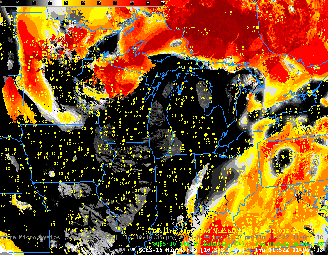
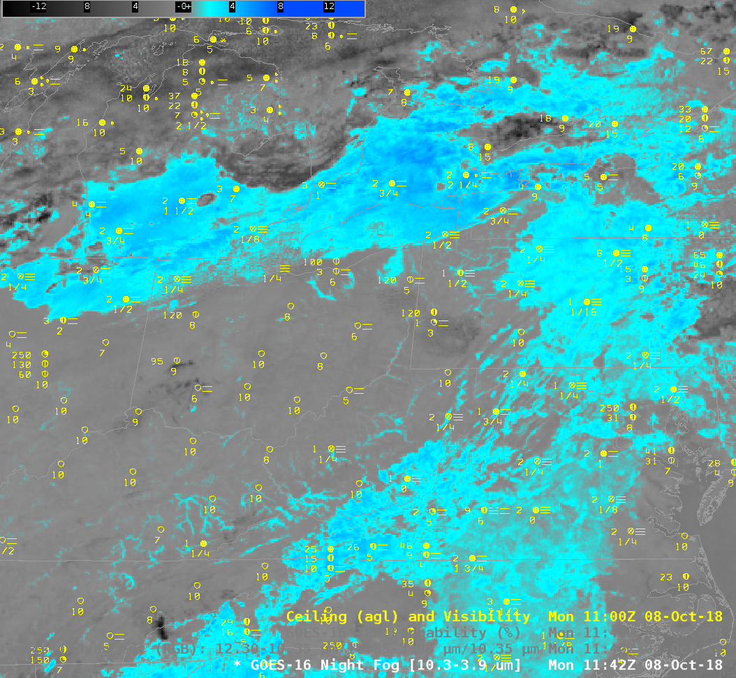
Consider the imagery above: The Night Fog Brightness Temperature Difference (10.3 µm – 3.9 µm) product can be used to highlight regions of low clouds (cloud made up of water droplets) because those water droplets do not emit 3.9 µm radiation as a blackbody (but do emit 10.3 µm radiation nearly as a blackbody), and the conversion of sensed radiance to brightness temperature assumes blackbody emissions. Thus, the 10.3 µm brightness temperature is warmer than at 3.9 µm. In the enhancement used, low stratus clouds are shades of cyan. Is there fog/low stratus along the coast of the Pacific Northwest? How far inland does it penetrate. It is impossible in this case (and many similar cases) to tell from satellite imagery alone because multiple cloud layers associated with a storm moving onshore prevent the satellite from seeing low clouds. The animation shows the Brightness Temperature Difference field along with surface reports of visibility and ceilings. IFR and near-IFR conditions are widespread, but there is little correlation between their location and the satellite-only signal.
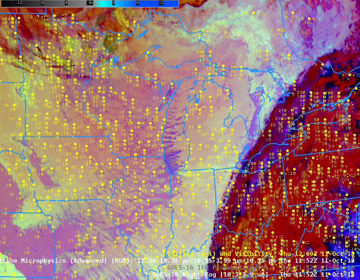
GOES-16 Night Fog Brightness Temperature Difference (10.3 µm – 3.9 µm), 1137 – 1452 UTC on 31 October 2018, along with surface reports of ceilings (AGL) and visibility (Click to animate)
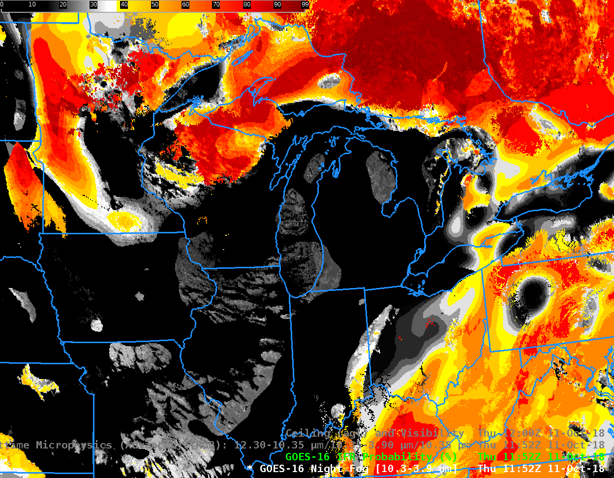
GOES-R IFR Probability fields fuse together satellite information and model data to provide a better estimate of where IFR conditions might be occurring. The animation below, for the same times as above, shows a high likelihood of IFR conditions (as observed) over much of the eastern third of Washington State. The satellite doesn’t give information about the near-surface conditions in this case, but the Rapid Refresh data strongly suggests low-level saturation, so IFR probabilities are high. The field also correctly shows small likelihood of IFR probailities over coastal southern Oregon and northern California. The Rapid Refresh data used have 13-km resolution, however; fog at scales smaller than that may be present — in small valleys for example.
GOES-16 IFR Probabilities, 1137 – 1452 UTC on 31 October 2018 (Click to animate)

