Category Archives: Southeast

Fog around Tampa Bay

The animation below shows IFR Probability fields layered on top of visible imagery. Early morning fog that reduced visibilities and ceilings to sub-IFR conditions are indicated over much of the middle of the Florida peninsula. (Note that the IFR Probabilty color enhancement was altered so that it was transparent for values < 20%, allowing the visible imagery beneath to appear).

GOES-16 IFR Probability Fields and Visible Band 2 (0.64 µm) imagery, 1151 – 1506 UTC (Click to enlarge)

GOES-16 Cloud Thickness fields, below, depict a shallow fog: thickness values in general are under 1000 feet. This scatterplot relates the last pre-sunrise Cloud Thickness — in meters! — to burn-off time; a value of 1000 feet will burn off very quickly as observed above.

Cloud Thickness at 1201 UTC on 23 February 2022 (Click to enlarge)

This website includes forecasts of visibility over Tampa Bay (and there are links to other coastal regions). The forecast below, for 1400 UTC 23 February / 0900 EST 23 February, has a maximum in predicted low visibility probability in about the right location. This forecast for the 24th suggests fog will be mostly offshore on the 25th.

Probability of low visibilities over/around Tampa Bay, valid 0900 EST on 24 February 2022 (Click to enlarge)

Fog over the southeast US

Low pressure just off the coast of South Carolina (0900 UTC map analysis) brought wide-spread fog and low ceilings to the southeastern United States on 7 February. The toggle below shows the Night Fog Brightness Temperature Difference (BTD, 10.3 µm – 3.9 µm) field that is often used to highlight regions where clouds made up of water droplets are widespread. The night time microphysics RGB includes as its green component the Night Fog BTD, and the correlation between the blue/cyan enhancement in the BTD and the cyan/yellowish color in the RGB is obvious. A challenge in using those two fields for low fog/stratus detection arises where multiple cloud layers might exist such that the BTD is not highlighting low cloud — because mid-level or high clouds block the satellite view of low clouds. This shortcoming is mitigated in IFR Probability fields by including information (from the Rapid Refresh model) on low-level saturation. Thus, IFR Probability fields suggest a greater likelihood for low clouds over coastal South Carolina (for example). If low-level saturation is *not* indicated in the model, IFR Probabilities will show minimal values, as over central Georgia (near Atlanta, especially), for example.

GOES-16 Night Fog Brightness Temperature Difference (10.3 µm – 3.9 µm), Night time microphysics RGB, and GOES-R IFR Probability, 1026 UTC on 7 February 2022 (Click to enlarge)

At 1156 UTC, a similar distribution to the three fields continues. Note how the presence of cirriform clouds over south-central Georgia affects the fields. The Night Fog BTD and Night Microphysics RGB both change radically, and IFR probabilities reduce — in part because the algorithm is less confident that low clouds exist. The small IFR Probabilities continue around Atlanta’s airline hub, important information from an aviation standpoint!

GOES-16 Night Fog Brightness Temperature Difference (10.3 µm – 3.9 µm), Night time microphysics RGB, and GOES-R IFR Probability, 1156 UTC on 7 February 2022 (Click to enlarge)

The toggle below compares IFR Probability with GOES-R Cloud Thickness. This is close to the time around sunrise/sunset when GOES-R Cloud Thickness are not computed because of quickly changing reflected solar shortwave infrared (3.9 µm) radiation; indeed, the cutoff can be viewed in the SSW-NNE terminator line over the Atlantic at the eastern edge of this image. If the low clouds on this day were strictly radiation (a dubious claim in the presence of rain!), then this scatterplot could be used to help decide when conditions might clear.

GOES-R IFR Probability and GOES-R Cloud Thickness fields, 1156 UTC on 7 February 2022 (Click to enlarge)

Coastal fog under clouds in South Carolina

GOES-16 Brightness Temperature Difference (10.3 µm – 3.9 µm), 0831 – 1331 UTC 1 March 2021 (Click to enlarge)

GOES-16 Night Fog Brightness Temperature Difference (BTD) fields (10.3 µm – 3.9 µm), above, show different cloud types in and around South Carolina before and through sunrise on 1 March 2021. Before sunrises, low clouds — stratus and fog — are characterized by blue/cyan/aqua colors in this enhancement. The positive brightness temperature difference arises because of emissivity differences in small cloud droplets for shortwave (3.9 µm) and longwave (10.3 µm) infrared radiation. Negative brightness temperature differences occur for higher clouds.

The presence of high clouds interferes with the satellite’s ability to view low clouds. Although one can infer a low cloud’s presence from an animation (and the assumption that the cloud doesn’t substantively change when a high cloud overspreads it), it’s a bit more difficult to extrapolate the cloud base from the cloud top behavior. In other words: Are the low clouds highlighted actually fog? Note also how the BTD enhancement changes as reflected solar radiation around sunrise starts to overwhelm any differences attributable to emissivity.

IFR Probability fields, shown below, combine the strength of satellite detection of low clouds with the strength model depiction of low-level saturation. IFR Probabilities will be quite high where satellites detect low clouds, and where Rapid Refresh model simulations show near-surface saturation. But if high clouds are in the way, IFR Probabilities can still be large if the Rapid Refresh model shows low-level saturation. This is occurring off the coasts of South and North Carolina. Note also: IFR Probability fields aren’t changing radically as the sun rises.

GOES-16 IFR Probability, along with surface observations of ceilings and visibility, 0831 UTC – 1326 UTC 1 March 2021 (Click to enlarge)

Night Fog Brightness Temperature Difference, Night time microphysics RGB, GOES-16 IFR Probability, 1001 UTC on 1 March 2021 (Click to enlarge)

The toggle above compares the Night Fog BTD with the Night time microphysics RGB (an RGB that takes as its green component the Night Fog BTD), and the GOES-16 IFR Probability fields at 1001 UTC on 1 March, shortly before sunrise. There is an obvious relationship between the RGB color and the regions of low clouds highlighted in the BTD by blue/cyan/aqua colors; the color of the RGB is tempered by the cloud temperature, however: the blue component of the RGB is the longwave infrared brightness temperature, and that is different over the ocean compared to over southwestern Georgia (for example). Note also how IFR Probability shows large values under the deep clouds over northwest South Carolina/western North Carolina.

Why is fog occurring offshore? Moist air over South Carolina is moving over relatively cool shelf waters, and cooled to its dewpoint; advection fog is the result. The toggle below shows surface dewpoints in the low 60s over coastal South Carolina. Sea-surface temperatures, shown at bottom from VIIRS at 0700 UTC and GOES-16 at 1300 UTC, show cool shelf waters with surface temperatures in the 50s (F).

GOES-16 IFR Probability with surface observations of ceilings/observations and surface METARs, 1001 UTC on 1 March 2021 (Click to enlarge)

NOAA-20 ACSPO VIIRS Sea Surface Temperatures (0701 UTC) and GOES-16 SST Temperatures (1301 UTC), click to enlarge

Cloud Layers and Detection of IFR Conditions

GOES-16 Night Fog Brightness Temperature Difference (10.3 µm – 3.9 µm), Nighttime Microphysics RGB and GOES-16 IFR Probability at 1116 UTC on 22 February 2019; Surface observations of ceilings and visibilities at 1100 UTC are also plotted (Click to enlarge).

A strong storm embedded within a subtropical jet stream over the southern United States was associated with widespread fog on the morning of 22 February 2019. This screen-capture from this site shows Dense Fog Advisories over much of Georgia, and over regions near Dallas. Which products allowed an accurate depiction of the low ceilings and reduced visibilities?

The toggle above cycles between the Night Fog Brightness Temperature Difference (10.3 µm – 3.9 µm), which product identifies low clouds (cyan blue in the default AWIPS enhancement shown) because of differences in emissivity at 3.9 µm and 10.3 µm from small water droplets that make up stratus clouds, the Nighttime Microphysics RGB, which RGB uses the Night Fog Brightness Temperature Difference as it green component, and the GOES-16 IFR Probability product. IFR conditions are defined as surface visibilities between 1 and 3 miles, and ceiling heights between 500 and 1000 feet above ground level. The plotted observations help define where that is occurring. Multiple cloud layers from Arkansas east-northeastward make a satellite-only detection of IFR conditions challenging. IFR Probability gives useful information below cloud decks because model-based saturation information from the Rapid Refresh Model fill in regions below multiple cloud decks where satellite information about low clouds is unavailable.

The toggle below shows the same three satellite-based fields (Night Fog Brightness Temperature Difference, Nighttime Microphysics RGB and IFR Probability) at the same time, but centered over Oklahoma. In this case, the Rapid Refresh Data are used to screen out a region of elevated stratus over northeast Oklahoma. Note that these is little in the Night Fog Brightness Temperature Difference field to distinguish between the IFR and non-IFR locations.

GOES-R IFR Probability over the southeast United States in this case is identifying regions of IFR conditions underneath multiple cloud decks (and also where only the low clouds are present) by incorporating low-level saturation information from the Rapid Refresh model. Over Oklahoma, non-IFR conditions under an elevated stratus deck are identified (and screened out in IFR Probability fields) by the lack of low-level saturation information in the Rapid Refresh.

Fog Detection Methods when Cirrus Clouds are present

GOES-R IFR Probability fields, 0545, 0800, 1000 and 1300 UTC on 13 June 2017 (Click to enlarge)

GOES-16 data posted on this page are (still!) preliminary, non-operational data and are undergoing testing

Note: GOES-R IFR Probabilities are computed using Legacy GOES (GOES-13 and GOES-15) and Rapid Refresh model information; GOES-16 data will be incorporated into the IFR Probability algorithm in late 2017

Reduced visibilities and lowered ceilings — IFR and Low IFR conditions — occurred over a wide stretch of the southeastern United States on the morning of 13 June 2017. The animation above shows enhanced IFR Probabilities aligned northwest to southeast from central Alabama to northwest Florida, the region where IFR Conditions develop. The flat nature of the field suggests that satellite data are not widely available as a predictor for low clouds on this morning, and that is because of widespread cirrus clouds over the southeastern United States (Click here to see the 0545 and 1300 UTC GOES-13 Water Vapor Imagery with cold brightness temperatures over the southeast). When high clouds are present, satellite-only detection of low clouds is not feasible.

For example, the brightness temperature difference field from GOES-13 (3.9 µm – 10.7 µm), below, has little predictive value for the northwest-to-southeast-oriented feature of low clouds/reduced visibilities because cirrus clouds are blocking the view.

GOES-13 Brightness Temperature Difference (3.9 µm – 10.7 µm) at 0545, 0800, 1000 and 1315 UTC on 13 June 2017 (Click to enlarge)

Various other detection techniques that rely on only satellite data similarly will be challenged by the presence of high clouds. For example, the Nighttime Microphysics RGB (From this site) shows little signal of fog (cyan/white in the RGB composite) over Georgia and Florida. Intermittent signals will appear occaionally as high clouds thin to allow the low-cloud signal through. The GOES-16 Brightness Temperature Difference field (10.33 µm – 3.9 µm) similarly is challenged by the presence of high clouds. The example shown at 1300 UTC shows a negative value because of reflectance off of high clouds.

Because the IFR Probability fields include surface information in the form of output from the Rapid Refresh model (saturation in the lowest part of the model is used as a predictor for the presence of fog), IFR Probability fields can fill in regions where satellite data cannot be used to detect low clouds because of the presence of high clouds. In regions where high clouds are present, satellite-only detection of fog and low stratus will always be a challenge.

Dense Fog over the Tennessee River Valley

GOES-R IFR Probabilities, 0100-1315 UTC on 25 April 2017 (Click to enlarge)

Dense Fog Advisories were issued over the Tennessee River Valley on Tuesday 25 April. The National Weather Service Aviation Weather website highlighted the regions of IFR conditions shortly after sunrise. IFR Probability fields, above, showed a slow increase in probabilities as ceilings and visibilities lowered during the night. The field outlined the region where IFR conditions were developing/occurring, meaning that it was a good situational awareness tool as the fog developed.

Brightness Temperature Difference fields, below, have historically been used to detect low clouds and by implication, fog. Clouds composed of water do not emit 3.9 µm radiation as a blackbody in contrast to their emissions of 10.7 µm radiation that are more like that of a blackbody. Thus, computed brightness temperature values are colder using 3.9 µm radiation than 10.7 µm radiation over water clouds. In the animation below, Brightness Temperature Difference values cooler than -1 C are highlighted in yellow.

Note that High Clouds in the animation below over the Smoky Mountains prevent an accurate depiction of low clouds formation there. IFR Probability fields, at top, include a signal in that region because model data from the Rapid Refresh model suggests saturation is occurring.

As the sun rises, at the end of the animation below, increasing amounts of reflected 3.9 µm radiation cause the brightness temperature difference field to flip in sign. In contrast, the IFR Probability fields, at top, maintain a coherent signal through sunrise.

Alert readers may note that Brightness Temperature Difference fields and IFR Probabilities are not shown from 0400 UTC. At that time, Stray Light signals were present in the Brightness Temperature Difference field and they contaminated both the Brightness Temperature Difference and the IFR Probability fields.

GOES-13 Brightness Temperature Difference (3.9 µm – 10.7 µm) from 0100 through 1315 UTC on 25 April 2017 (Click to enlarge)

GOES-16 is transmitting non-operational data that are undergoing testing and refinement. The toggle below shows the brightness temperature difference field from GOES-16 and GOES-13 for one time on 25 April. Note the superior resolution in the GOES-16 data: 2 km at the subsatellite point vs. 4 km for GOES-13. As noted at the start of this blog post, GOES-R IFR Probabilities are being computed with GOES-13 and GOES-15 data, not with GOES-16 data. Incorporation of GOES-16 data into the algorithm will occur near the end of 2017.

The GOES-16 data posted on this page are preliminary, non-operational data and are undergoing testing.

GOES-16 and GOES-13 Brightness Temperature Difference fields, 1300 UTC on 25 April 2017 (Click to enlarge)

Dense Fog over the Carolinas

GOES-13 Brightness Temperature Difference (3.9 µm – 10.7 µm), GOES-R IFR Probability and GOES-R Cloud Thickness at 1115 UTC on 17 January 2017 (Click the enlarge)

Dense Fog Advisories (National Weather Service Website) and IFR SIGMETs (Aviation Weather website) were issued early in the morning for dense fog over the southeastern United States. The toggle above from 1115 UTC on 17 January shows the Brightness Temperature Difference field (3.9 µm – 10.7 µm), the GOES-R IFR Probability Field, and the GOES-R Cloud Thickness fields associated with this dense fog event. Note the presence of high clouds over northern South Carolina and western North Carolina — the dark region in the Brightness Temperature Difference enhancement — prevents the brightness temperature difference field from highlighting that region of reduced ceilings/visibilities. The GOES-R Cloud Thickness field is not computed under cirrus either, as it relates 3.9 µm emissivity of water-based clouds to cloud thickness (based on a look-up table generated using data from a SODAR off the West Coast of the United States). If cirrus blocks the view, then, neither the Brightness Temperature Difference field nor the GOES-R Cloud Thickness field can give useful information about low clouds.

In contrast, the GOES-R IFR Probability field does give useful information in regions where cirrus clouds (and low clouds/fog) are present — because Rapid Refresh information about the lower troposphere can be used. IFR Probability values will be smaller in those regions because satellite predictors are unavailable, and the Probability incorporates both predictors from satellites and from Rapid Refresh model output — if the satellite predictors are missing because of cirrus, the IFR Probability values will be affected. Despite the smaller values, however, the IFR Probability fields in regions of cirrus are giving useful information for this event.

GOES-R Cloud thickness fields can be used to estimate Fog dissipation using the last GOES-R Cloud Thickness field produced before twilight conditions at sunrise (shown below for this case). (GOES-R Cloud Thickness is not computed during twilight conditions because of rapidly changing 3.9 µm emissivity related to the reflected solar radiation as the sun rises, or as it sets). This scatterplot gives the relationship between thickness and dissipation time after the Cloud Thickness time stamp (1215 UTC in this case). In this case, the thickest fog is near Athens GA; the algorithm predicts that clearing should happen there last, at about 1515 UTC.

GOES-R Cloud Thickness, 1215 UTC on 17 January 2017 (Click to enlarge)

Dense Fog in Georgia and Florida

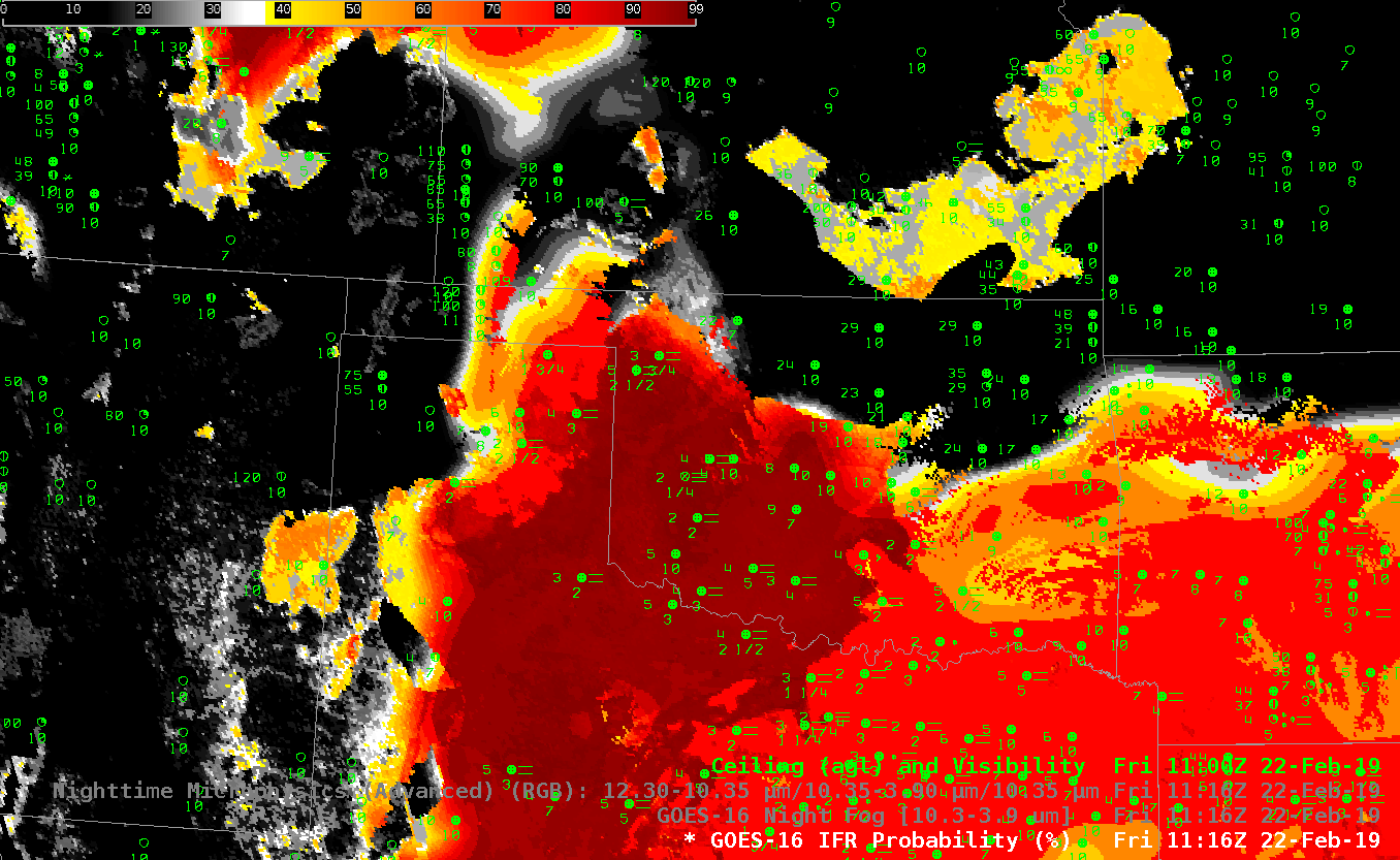
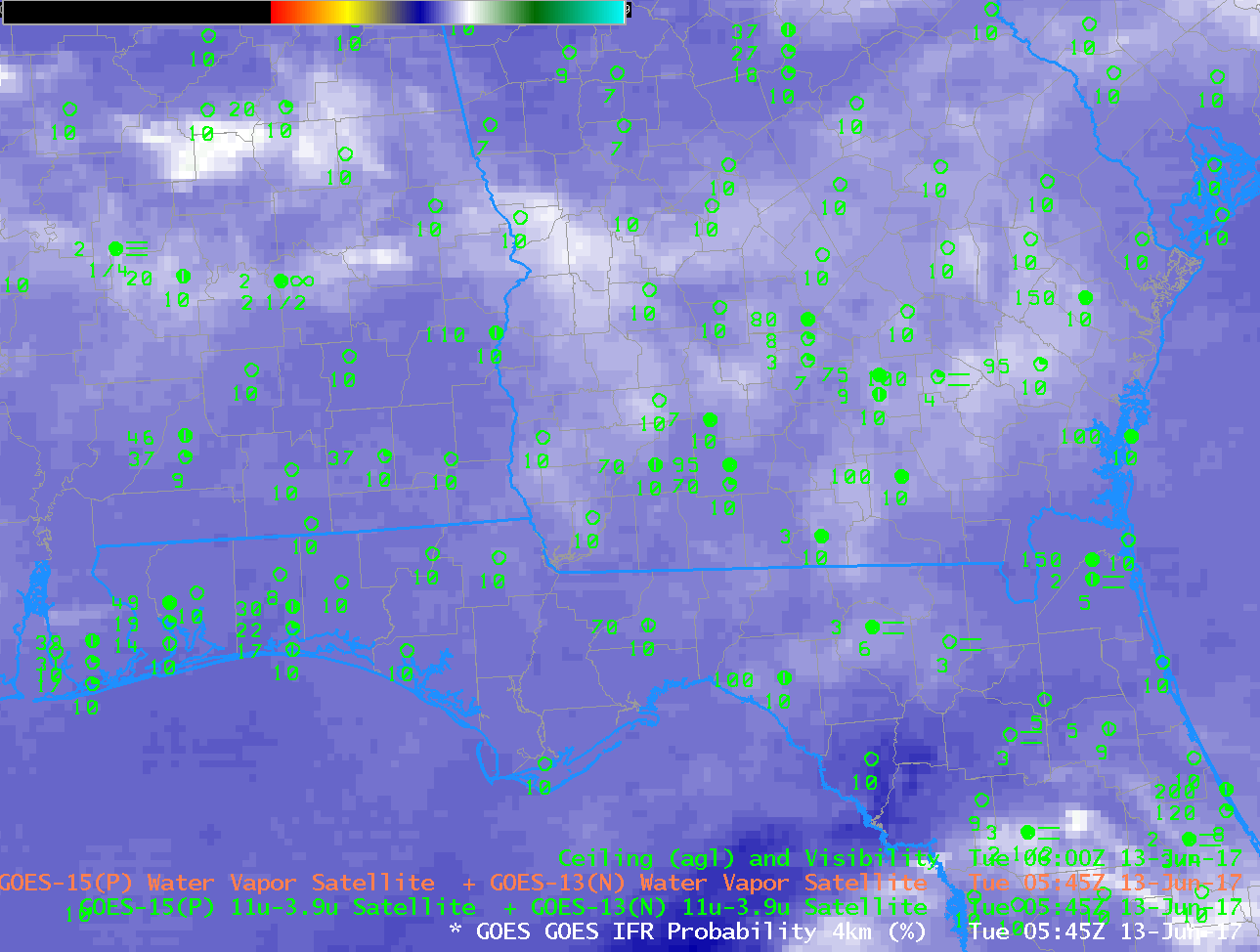
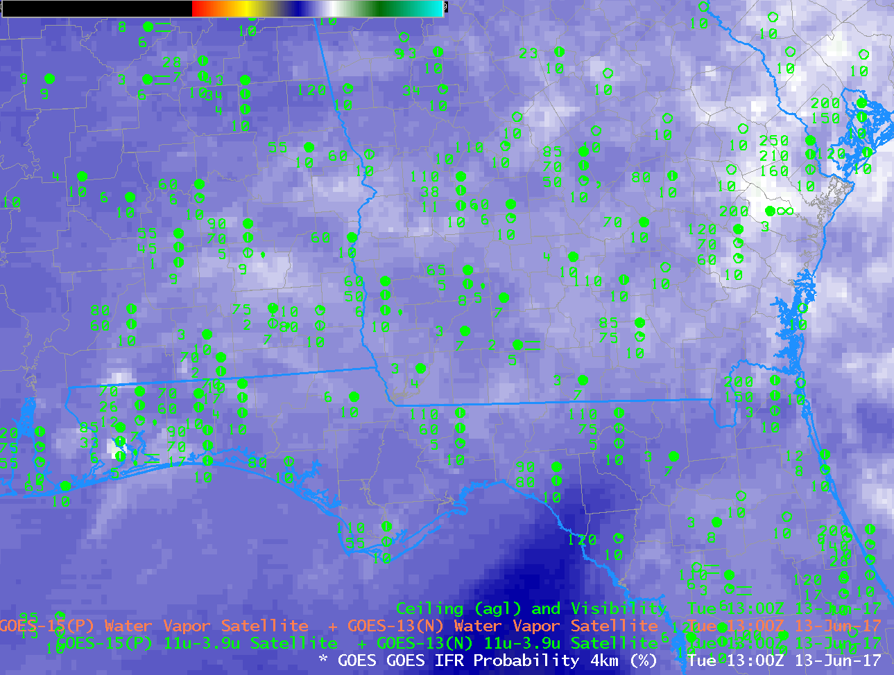
GOES-R IFR Probability Fields, 0000 – 1300 UTC on 25 November 2016 (Click to enlarge)

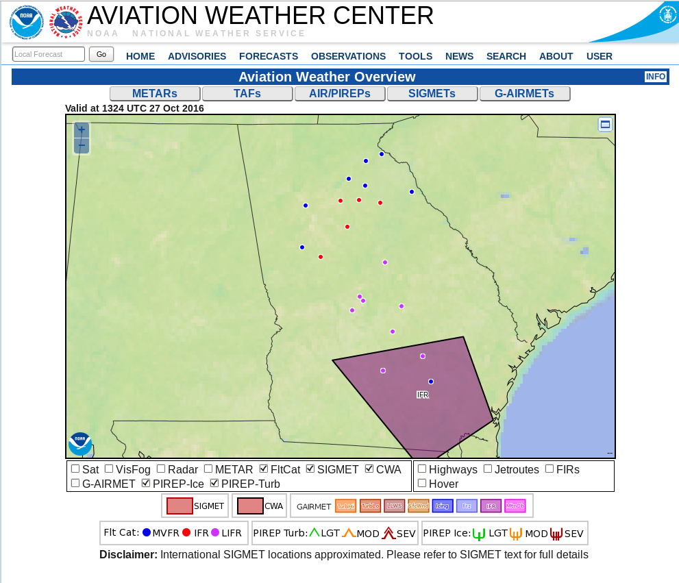
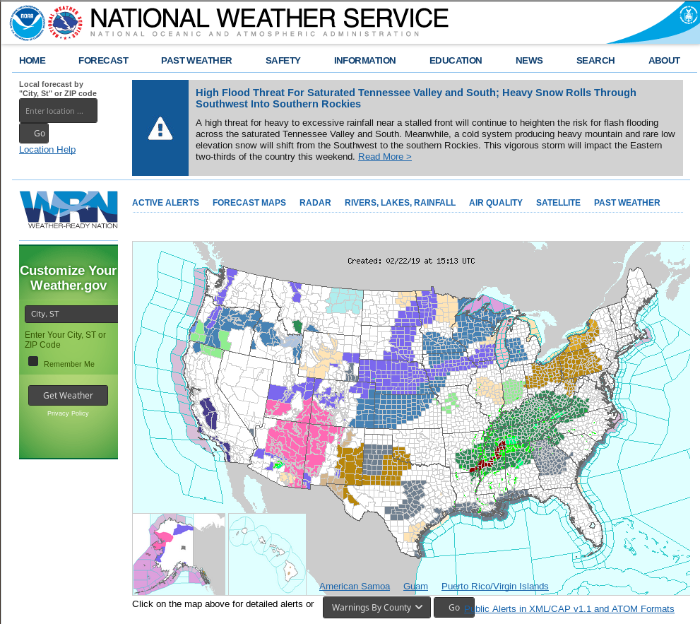
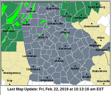
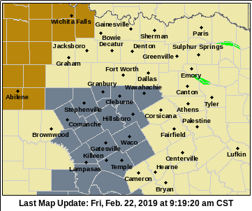
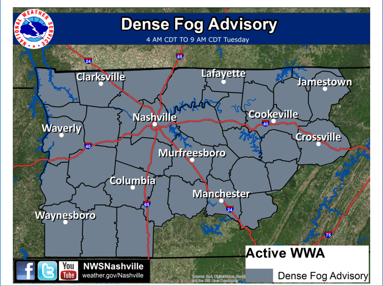
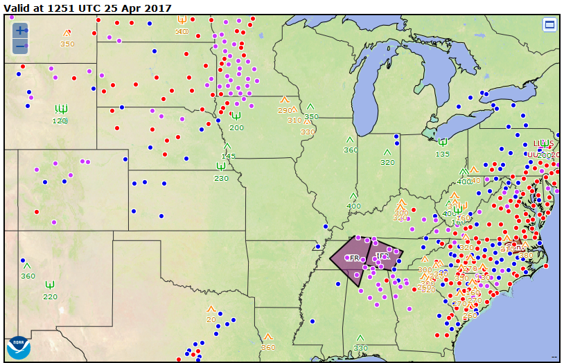
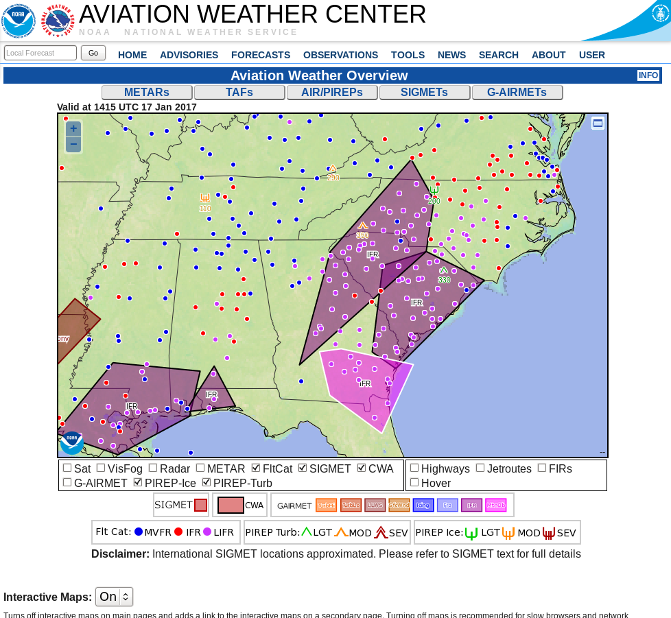
Light winds and a long November night allowed radiation fog formation over much of the deep south early on 25 November 2016. (1200 UTC Surface analysis is here). The Aviation Weather Center Website indicated widespread IFR Conditions, below, over the south, with the sigmet suggesting improving visibilities after 1400 UTC.

The animation above shows the evolution of the GOES-R IFR Probability fields from just after sunset to just after sunrise. There is a good spatial match between observed IFR conditions and the developing field. IFR Probability can thus be a good situational awareness tool, identifying regions where IFR Conditions exist, or may be developing presently.

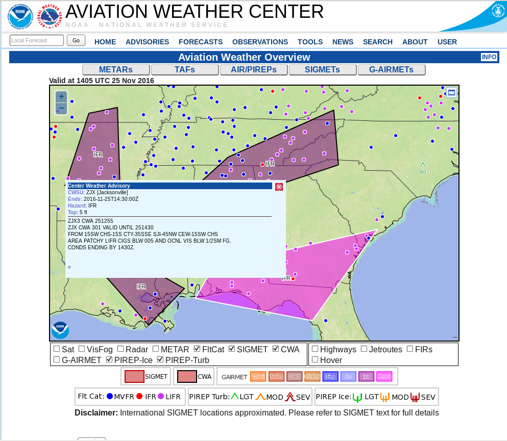
Screenshot of Aviation Weather Center Front Page, 1405 UTC on 25 November (Click to enlarge)

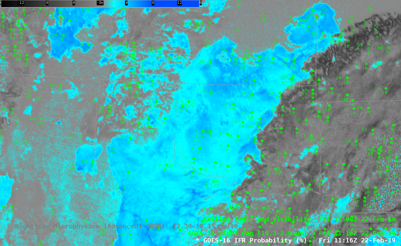
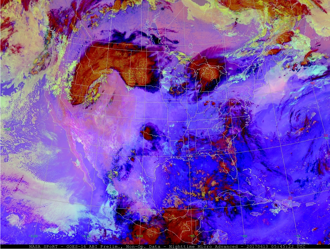
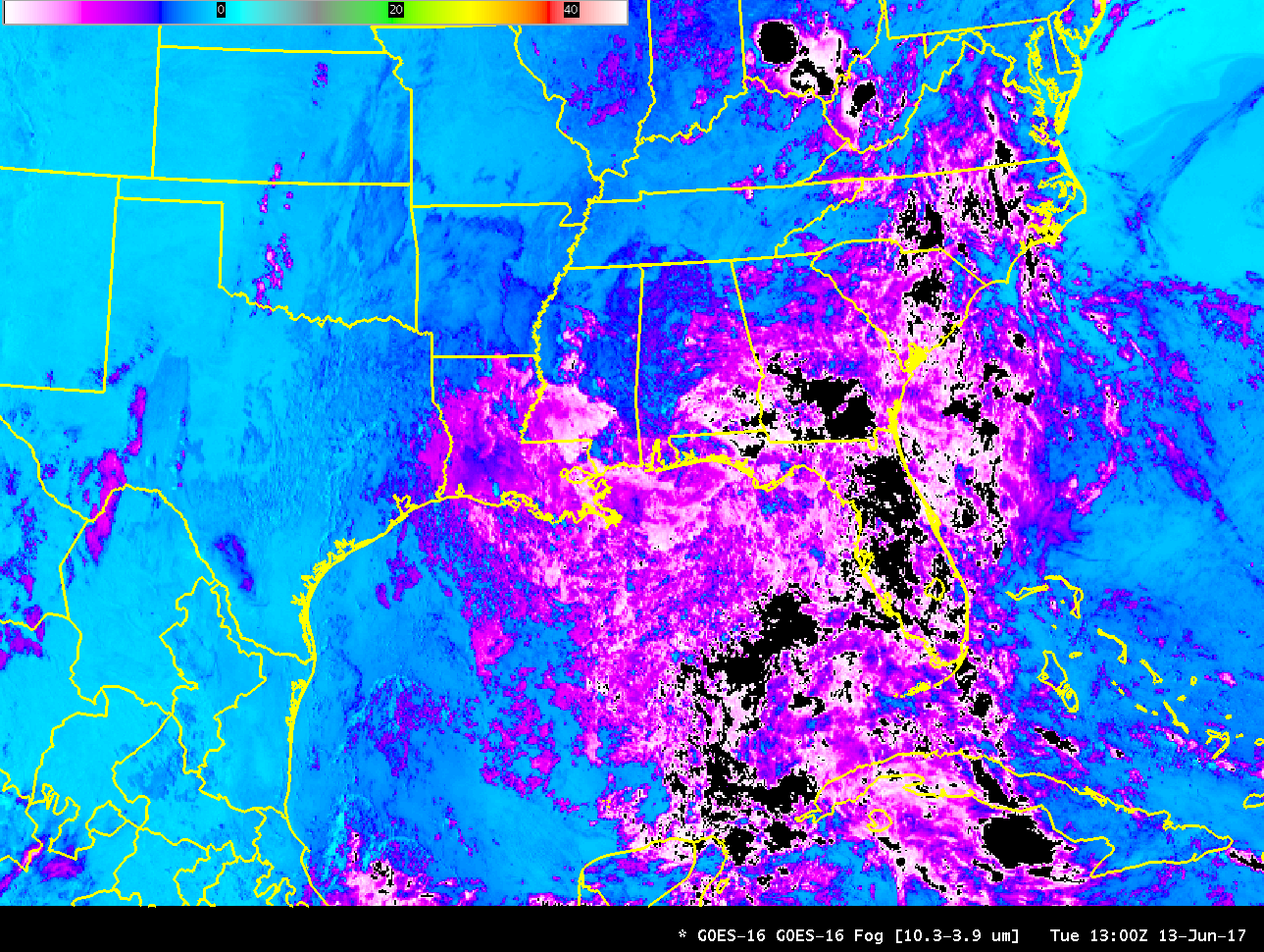
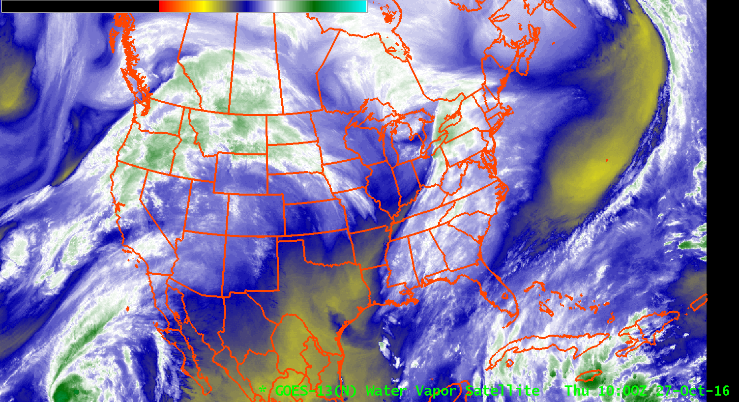
Did the GOES-13 Brightness Temperature Difference Field identify the fields? The animation below, from 0200-1300 UTC, shows a widespread signal that shows no distinguishable correlation with observed IFR conditions. Note also how the rising sun at the end of the animation changes the difference field as more and more reflected solar radiation with a wavelength of 3.9 µm is present. In addition, high clouds that move from the west (starting at 0400 UTC over Louisiana) prevent the satellite from viewing low clouds in regions where IFR conditions exist.

GOES-13 Brightness Temperature Difference field (3.9 µm – 10.7 µm), 0200-1300 UTC on 25 November 2016 (Click to enlarge)

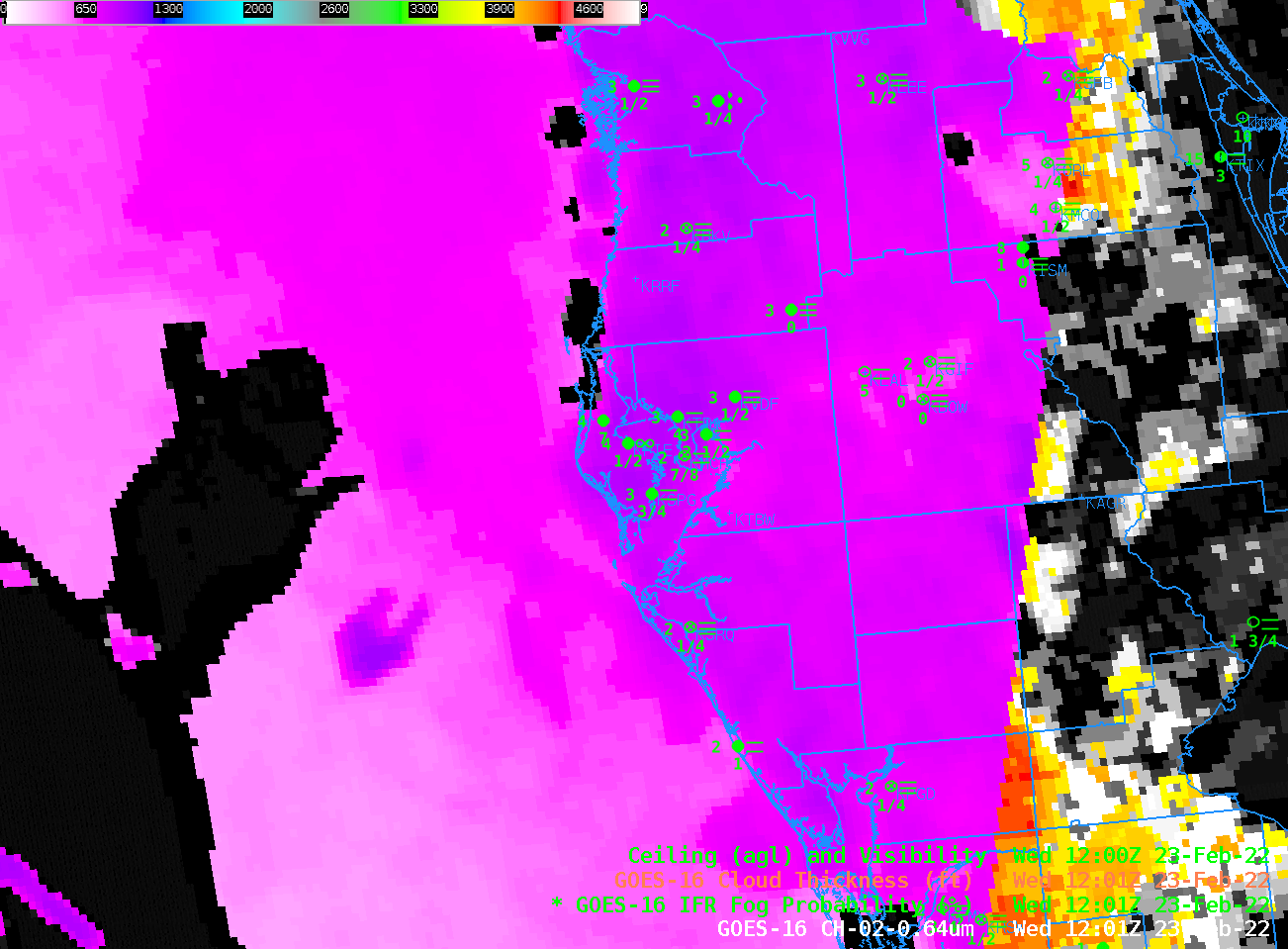
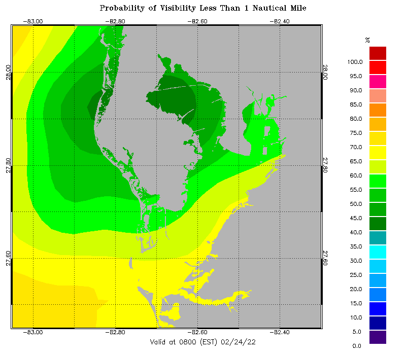
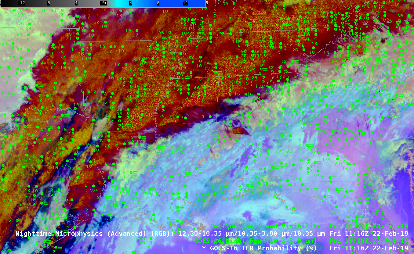
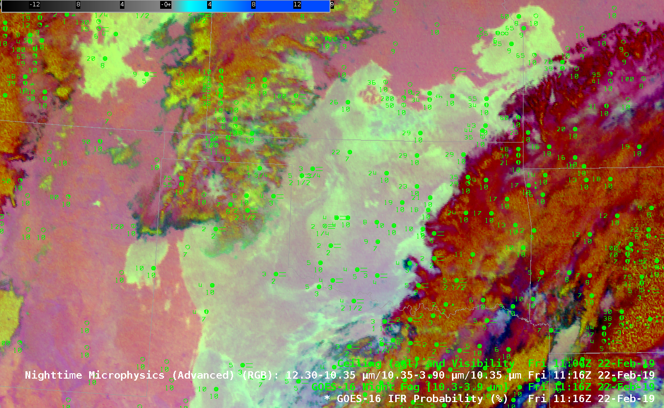
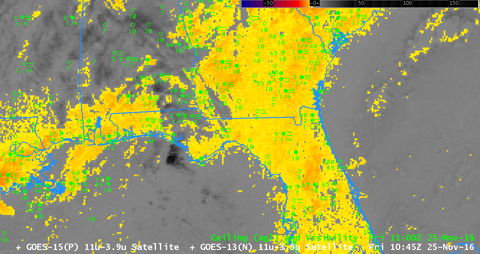
The high clouds that prevent satellite detection of low clouds, as for example at 1100 UTC over parts of Alabama, cause a noticeable change in the IFR Probability fields, as shown in the toggle below. Values over the central part of the Florida panhandle are suppressed, and the field itself has a flatter character (compared to the pixelated field over southern Georgia, for example, where high clouds are not present). Even though high clouds prevent the satellite from providing useful information about low clouds in that region, GOES-R IFR Probability fields can provide useful information because of the fused nature of the product: Rapid Refresh information adds information about low-level saturation there, so IFR Probability values are large. In contrast, over southern Florida — near Tampa, for example, Rapid Refresh data does not show saturation, and IFR Probabiities are minimized even through the satellite data has a strong signal — caused by mid-level stratus. Soundings from Tampa and from Cape Kennedy suggest the saturated layer is around 800 mb.

GOES-R IFR Probability fields and GOES-13 Brightness Temperature Difference Fields, 1100 UTC on 25 November 2016 (Click to enlarge)

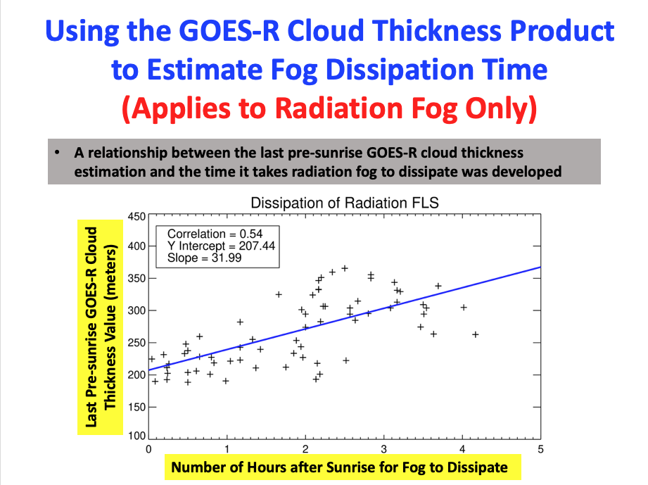
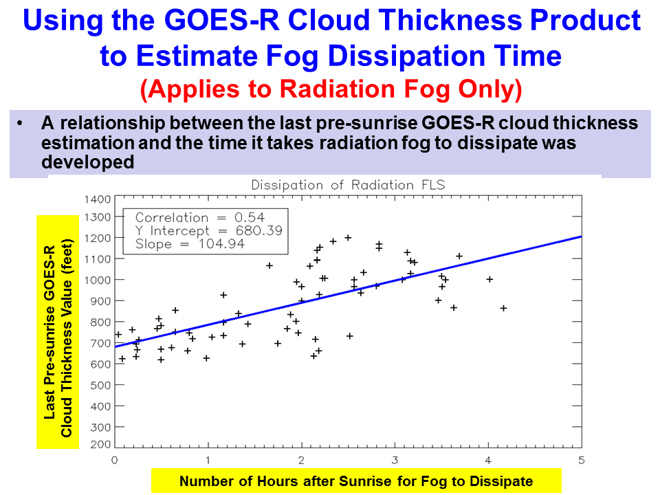
GOES-R Cloud Thickness, below, related 3.9 µm emissivity to cloud thickness via a look-up table that was generated using GOES-West Observations of marine stratus and sodar observations of cloud thickness. The last pre-sunrise thickness field, below, is related to dissipation time via this scatterplot. The largest values in the scene below are around 1000 feet, which value suggests a dissipation time of about 3 hours, or at 1445 UTC.

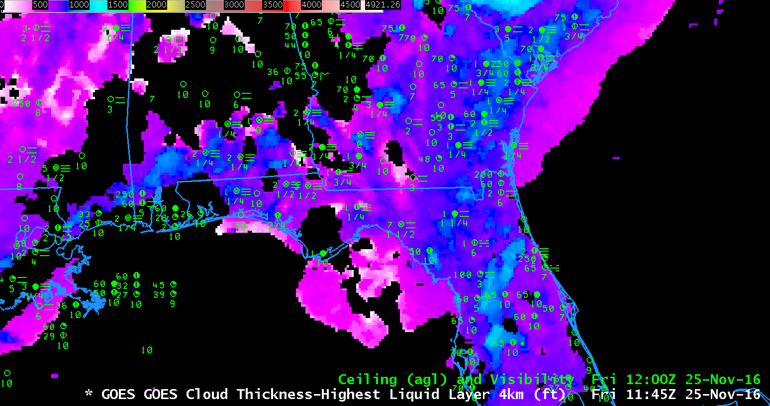
GOES-R Cloud Thickness Field, 1145 UTC on 25 November 2016 (Click to enlarge)

IFR Probability Fields let you peek beneath the Cirrus

GOES-13 Brightness Temperature Difference (3.9 µm – 10.7 µm) fields, hourly from 0215-1215 UTC on 27 October (Click to enlarge)

If you rely on satellite data alone to anticipate the development of IFR conditions — fog, low ceilings, and reduced visibilities — then the presence of widespread cirrus, shown here with the GOES-13 6.5 µm image, makes situational awareness difficult. At a glance, can you tell in the animation of brightness temperature difference, above, hourly from 0215 through 1215 UTC, where IFR Conditions are occurring? The widespread cirrus, present in the enhancement as dark grey and black, prevents the satellite from viewing any fog development, hence making this brightness temperature difference field, traditionally used to detect the development of fog and low stratus, unsuitable for large-scale situational awareness.

GOES-R IFR Probability fuses satellite data with Rapid Refresh Model output and allows a product that in essence peeks beneath the cirrus because near-surface saturation predicted in the Rapid Refresh Model allows the IFR Probability product to have a strong signal where fog might be developing. Consider the animation below, that covers the same spatial and temporal domain as the brightness temperature difference animation above. IFR Probability increases over inland southeast Georgia in concert with the development of low ceilings/reduced visibilities. It gave a few hours alert to the possibility that IFR conditions would be developing. Note in the animation below that the 1215 UTC image includes IFR Probabilities computed using daytime predictors and nighttime predictors. There is therefore a discontinuity in the field values over central Georgia at 1215 UTC, the end of the animation.

Compare the animation below to the one above. Which yields better situational awareness for the developing fog field?

GOES-R IFR Probability Fields, hourly from 0215 through 1215 UTC on 27 October (Click to enlarge)

The Aviation Weather Center plot (below) highlights the presence of an IFR SIGMET over the region at 1324 UTC on 27 October.

Aviation Weather Center plot showing MVFR, IFR and LIFR stations over Georgia, along with an IFR Sigmet at 1324 UTC 27 October 2016 (Click to enlarge)

IFR Probability Screens out mid-level Stratus

GOES-13 Brightness Temperature Difference (3.9 µm- 10.7 µm) and GOES-R IFR Probability fields computed with GOES-13 and Rapid Refresh Data, 1100 UTC 18 October. Plots of ceilings and surface visibilities are included (Click to enlarge)

GOES-R IFR Probability fields often to a better job (compared to brightness temperature difference fields) in outlining exactly where low ceilings and reduced visibilities are occurring because IFR Probability fields include information about low-level saturation from the Rapid Refresh model. That information about near-surface saturation allows the IFR Probability algorithms to screen out regions where only mid-level stratus is occurring. A low fog — a stratiform cloud of water droplets that sits on/near the surface — and a mid-level stratus deck (also a stratiform cloud of water droplets) can look very similar in a brightness temperature difference field. In the example above, consider much of northeastern Alabama and northern Georgia. There is a strong return in the brightness temperature difference field because mid-level stratus is present — but IFR Probabilities are small because the Rapid Refresh does not diagnose low-level saturation in the region. Compare Brightness Temperature Difference returns over northeast Alabama and over extreme western North Carolina — to the west of Asheville. IFR Conditions are observed over western North Carolina, and IFR Probabilities are high there. In general, the region with high IFR Probabilities in the toggle above includes stations that are reporting IFR or near-IFR conditions. Most stations outside the region of high IFR Probability are not showing IFR Conditions, even though they may be in a region with the Brightness Temperature Difference signal is large.

A similar story can be told farther west at 0800 UTC, shown below. Focus on the region with a strong Brightness Temperature Difference signal over southeast Arkansas. IFR Conditions are not occurring under that mid-level stratus deck, and IFR Probabilities are very low. Similarly, IFR Probabilities are small over Oklahoma and north-central Texas because the Rapid Refresh Model is not showing low-level saturation in those regions; IFR Probabilities cannot be large when low-level saturation is not indicated in the model.

Using both Satellite Data and Model Data accentuates the strengths of both. That’s the power of a fused data product.

GOES-13 Brightness Temperature Difference (3.9 µm – 10.7 µm) and GOES-R IFR Probability fields computed with GOES-13 and Rapid Refresh Data, 0800 UTC 18 October. Plots of ceilings and surface visibilities are included (Click to enlarge)

GOES-R Fog Product Examples

Fog detection fusing GOES, Terra/Aqua or Suomi/NPP Satellite data with Model output