Category Archives: Plains

Fog backed up against the front range of the Rockies

GOES-16 Night Fog Brightness Temperature Difference (10.3 µm – 3.9 µm) and Nighttime microphysics RGB, 0901 UTC on 11 May 2021, along with observations of ceilings (AGL) and visibility

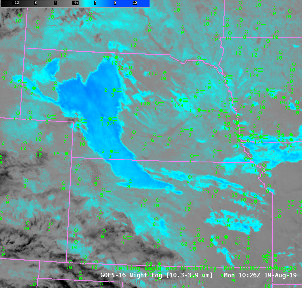
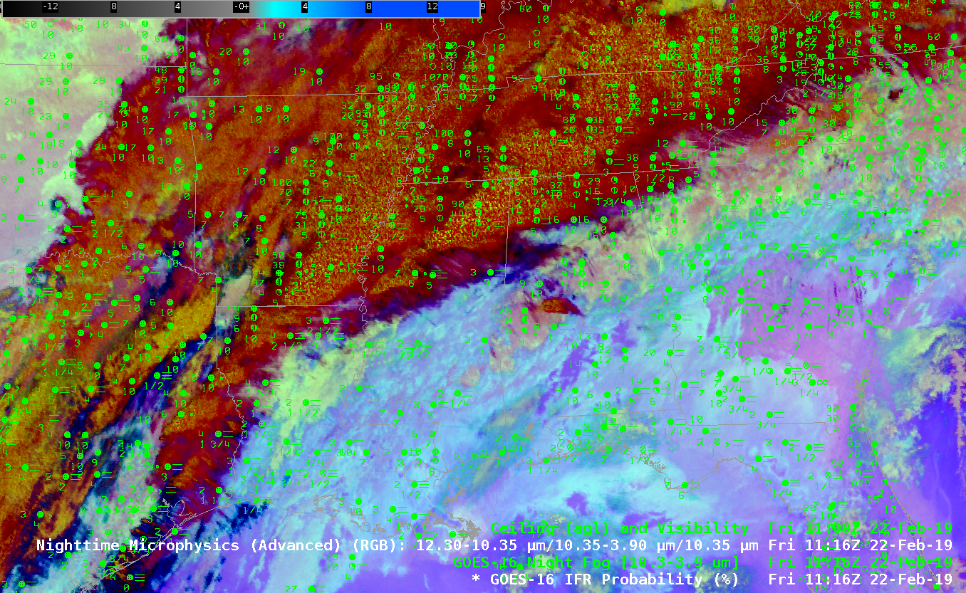
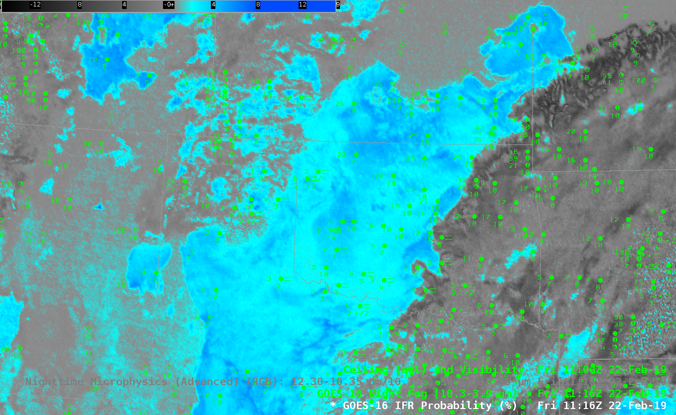
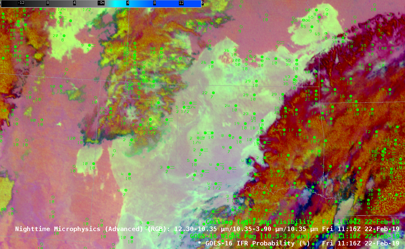
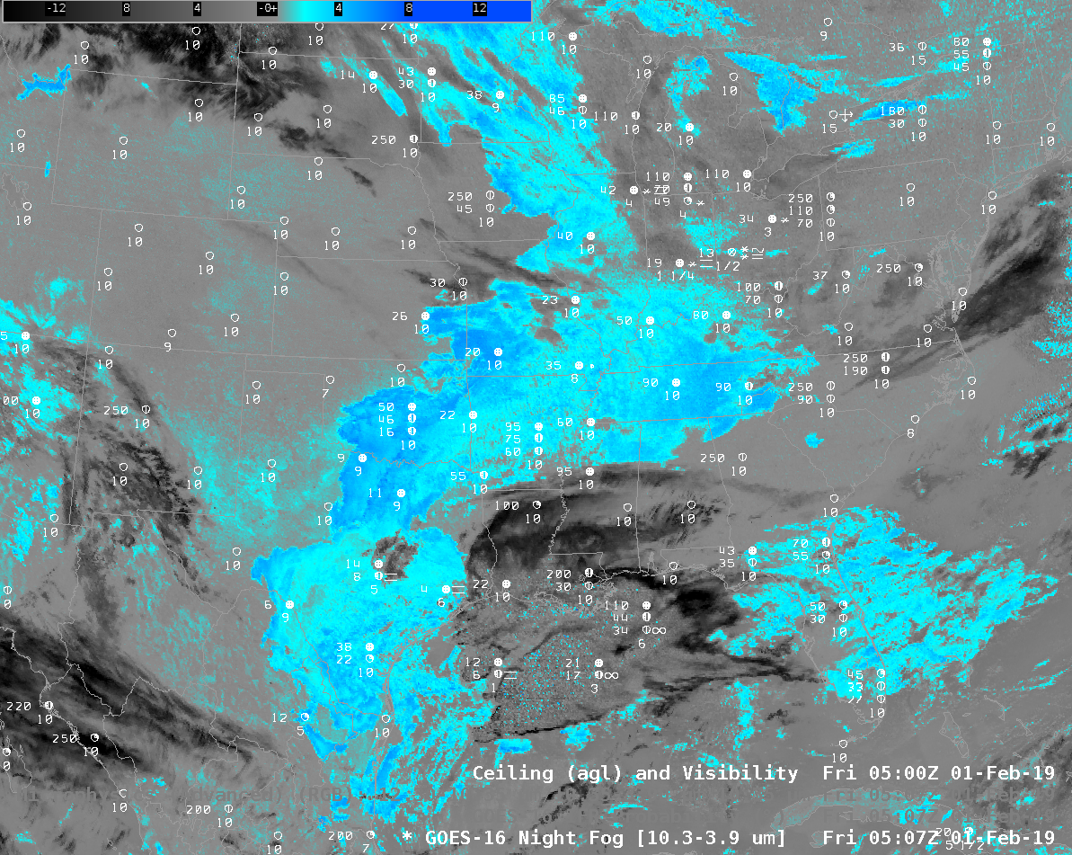
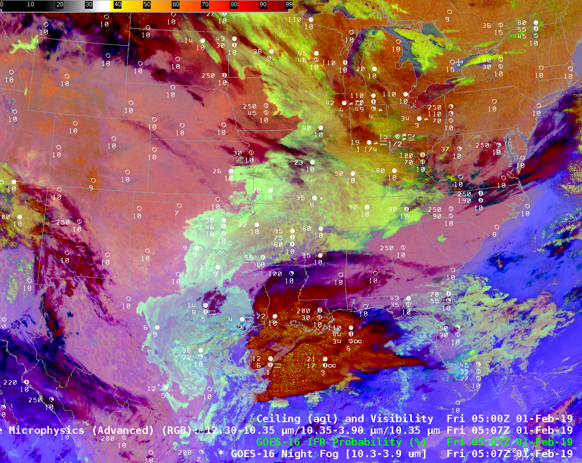
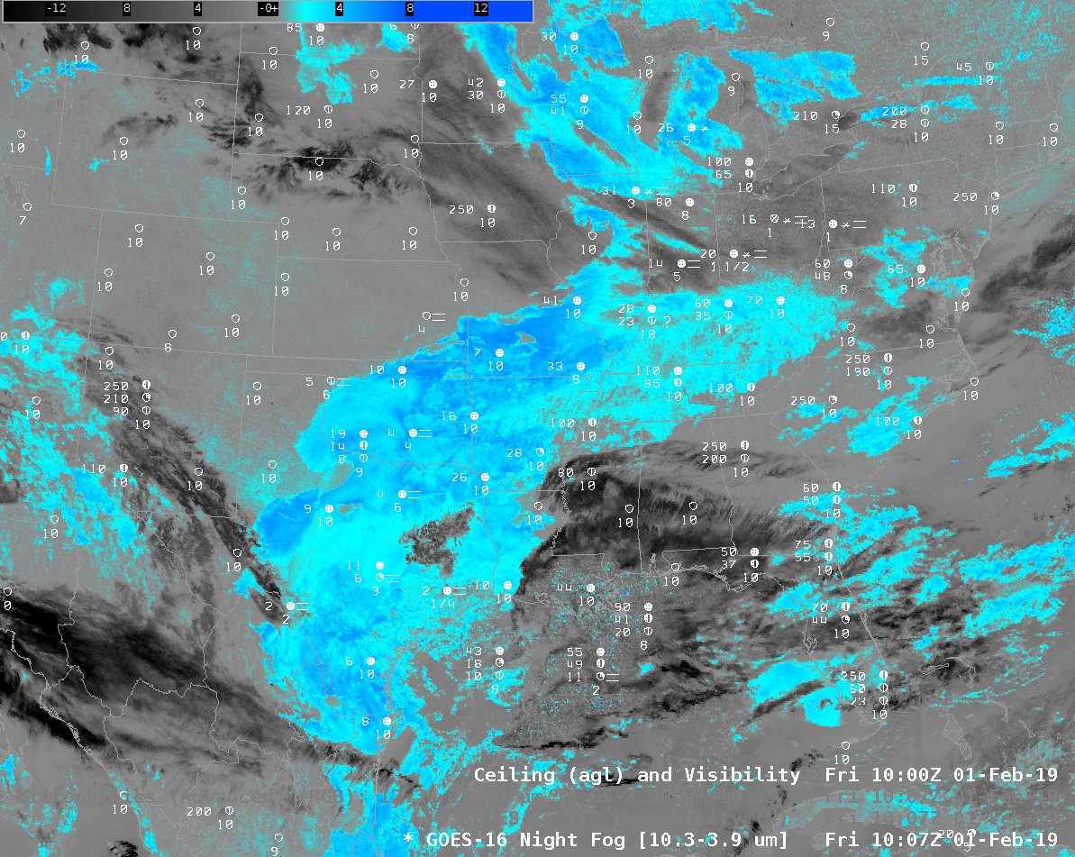
The toggle above compares Night Fog Brightness Temperature difference fields at 0901 UTC on 11 May over Colorado and surrounding states. Both fields can be used to identify regions of stratus/low stratus — and by inference, fog. At this time, however, it is a challenge to use these satellite-only products because of widespread mid/upper-level clouds over eastern Colorado, Kansas and Nebraska. Note how the blue/cyan regions in the Night Fog Brightness Temperature Difference field show through into the Nighttime Microphysics RGB; the green component of that RGB is the Night Fog Brightness Temperature Difference field.

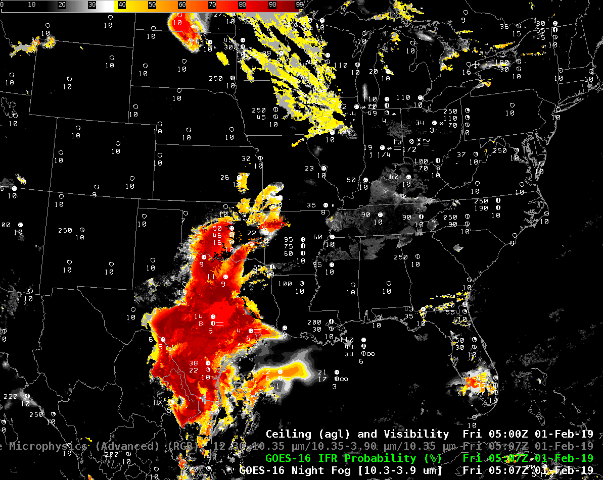
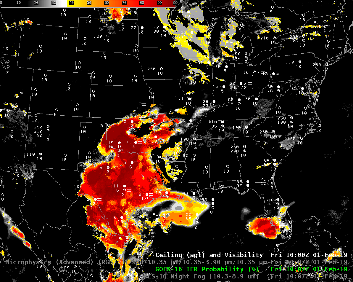
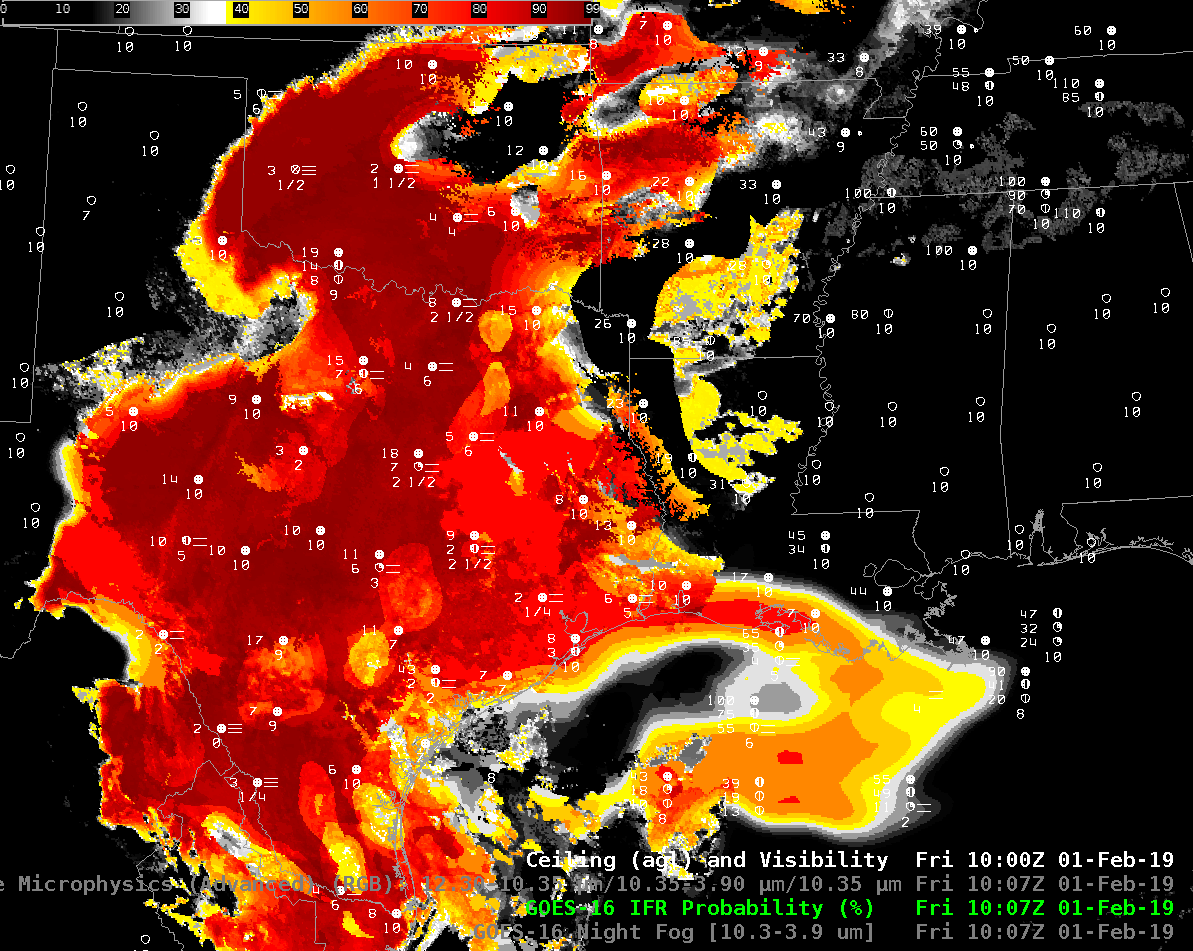
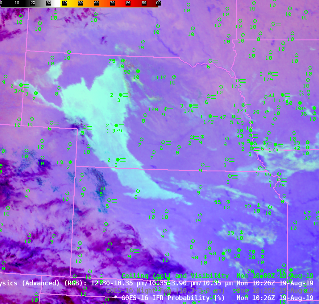
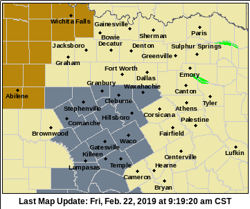
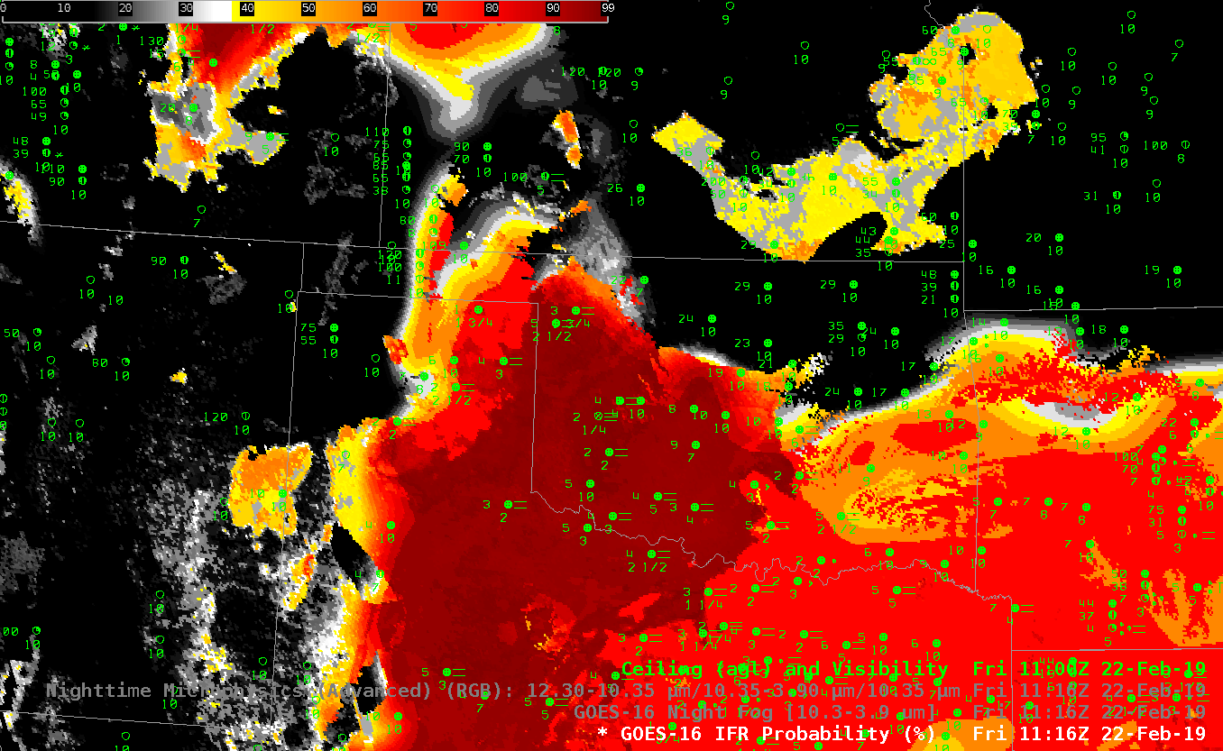
On this day, the high clouds prevented the Brightness Temperature Difference alone from highlighting regions of fog. IFR Probability fields, below from the same time, show that this field better outlined the region of low clouds/fog over the High Plains. The field incorporates both Night Fog Brightness temperature difference fields — to determine where stratus clouds might be — and Rapid Refresh model estimates of low-level moisture — to determine where saturation might be occurring. Where the satellite detects stratus clouds, and where the Rapid Refresh model suggests low-level saturation, high IFR Probability (as over southeastern Colorado) results, in accordance with, on this day, observations. If high clouds are present (as over much of eastern Colorado), IFR Probability can still occur because the Rapid Refresh data shows low-level saturation. Note also that the extensive cloud cover over Kansas and Nebraska — elevated stratus — does not have a strong signal in the IFR Probability fields.

This product blends the strengths of satellite observations and the strength of model estimates.

GOES-16 Night Fog Brightness Temperature Difference  (10.3 µm – 3.9 µm) and IFR Probability, 0901 UTC on 11 May 2021, along with observations of ceilings (AGL) and visibility

IFR Probability over Missouri

GOES-16 IFR Probability, 0646 – 1501 UTC on 19 January 2021 (Click to enlarge)

GOES-16 IFR Probability fields, above, show a gradual expansion southward of the regions of highest probability of reduced visibility. As the fields encroach over stations, visibilities and ceilings are reduced: there is a very good relationship between observed IFR conditions and enhanced IFR Probabilities. This field could be used on 19 January to predict the onset of low ceilings and reduced visibilities.

You will note that there are hourly changes to the IFR Probability fields. Rapid Refresh model data used in the computation of IFR Probability is updated each hour when a more recent model simulation is incorporated into the data. You can also identify regions where satellite data are not used because high clouds are preventing a satellite view of low stratus: there are regions where IFR probability is an unpixelated mostly uniform field.

The Night Time microphysics RGB for the same period, shown below, also highlights the region of low clouds as a cyan/yellow feature slowly moving southward. In principle, this field is only showing you that stratus clouds are present, because information about the cloud base (supplied by the Rapid Refresh model in IFR Probability fields) is lacking.

The challenge of using the Night Time Microphysics field is also apparent near the end as the Sun rises and the color associated with the stratus clouds changes.

GOES-16 Night Time Microphysics RGB, 0646 – 1501 UTC, 19 January 2021 (Click to enlarge)

The toggle below compares the GOES-16 IFR Probability field and the GOES-16 Night Time Microsphysics RGB at 1201 UTC. A cirrus shield along the southern boundary of the IFR Probability field is hindering the ability of the Night Time Microphysics RGB there to detect low clouds.

GOES-R IFR Probability and Night Time Microphysics, 1201 UTC on 19 January 2021 (Click to enlarge)

IFR Conditions over the southern Plains

Click to enlarge
GOES-16 Night Fog Brightness Temperature Difference (10.3 µm – 3.9 µm), Night TIme Microphysics RGB, and IFR Probability, 1001 UTC on 22 September 2020 (Click to enlarge)

Widespread mid- and upper-level cloudiness over the southern Plains associated with Tropical Storm Beta on 22 September 2020 make it difficult to use satellite data alone to identify where low clouds and fog might exist. This is a day where IFR conditions exist, as shown here, an image from this website. Where would you expect IFR conditions to exist within this field of view? The Night Fog brightness temperature difference, below, (and, by extension, the Nightime Microphysics RGB) shows scant information over eastern Texas/Oklahoma or ArkLaTex. IFR Probability fields, in contrast, have a definite signal of high probability.

The animation of the Night Fog Brightness Temperature Difference field, below, also highlights a challenge in using this product: increasing reflection of solar 3.9 radiation occurs as sunrise progresses, changing the character of the field. Further, soils can have emissivity properties that are similar to clouds, and a positive Night Fog Brightness Temperature difference signal results. (This is especially true in dry regions, such as west Texas; linked-to map from this website).

GOES-16 Night Fog Brightness Temperature Difference (10.3 µm – 3.9 µm), 0901 – 1306 UTC on 22 September 2020 (Click to enlarge)
GOES-16 IFR Probability, 0901-1306 UTC on 22 September 2020 (Click to enlarge)

IFR Probability fields for the same time as the Night Fog Brightness Temperature Difference, above, show a consistent region where IFR conditions are most likely. The region over the high Plains of Texas that has a signal in the Brightness Temperature Difference field has low probabilities because in that region, the Rapid Refresh model is not suggesting widespread low-level saturation. In contrast, the Rapid Refresh model over east Texas/Oklahoma, western Louisiana and southwest Arkansas does show saturation.

What do observations shows? The hourly observations overlain on the IFR Probability fields, below, show that IFR and near-IFR conditions are widespread within the region of high IFR Probability. Outside that region, IFR conditions are rare.

GOES-R IFR Probability fields, 0906, 1001, 1101, 1201 and 1301 UTC along with observations of ceilings and visibilities (Click to enlarge)

IFR Probability fields are flowing over the SBN to forecast offices. (TOWR-S RPM 19 is needed to display them from that data source). IFR Probability fields are also available via an LDM feed from Regionals if RPM 19 is not installed. They are available online at this website.

IFR conditions over the Great Plains

Surface Analysis at 0900 UTC on 13 May 2020

Much of the central Plains of the United States was under easterly flow during the night on 12-13 May 2020, as suggested by the surface analysis above. Strong High Pressure over the Great Lakes and lower pressures over the Rocky Mountains drove that upslope flow. Consequently, IFR conditions were common over much of the Plains, as shown below.

The animation, below, of IFR Probability (overlain with surface observations and ceilings and visibilities) shows high probabilities. There is good correlation between regions with High IFR Probabilities — red and orange — and regions with low ceilings and reduced visibilities. The highest probabilities, dark red in the enhancement, occur where satellite data shows low clouds and where model data shows low-level saturation. Note that there is a trend towards less satellite information in the IFR Probability field with time over central Oklahoma and south-central Kansas because of developing convection.

GOES-16 IFR Probability fields, 0800-1136 UTC on 13 May 2020

The night time microphysics RGB, shown below, is also used to detect regions of low clouds; they typically appear yellowish at this time of year. The challenge with the RGB use in highlighting IFR conditions is two-fold: high clouds will mask the low cloud signal (as in the case of developing convection over Oklahoma, or with cirrus over Colorado and Nebraska). The RGB can also struggle to differentiate between fog and low stratus. Note also in this animation how the effect of the rising sun becomes apparent at the end of the animation over the eastern third of the image.

Night time Microphysics RGB, 0801-1136 UTC on 13 May 2020

In the toggle below, the signal of low clouds in the RGB, yellow/cyan over the Texas panhandle (for example) has an echo in the IFR Probability field. In the absence of high clouds, both products will show regions of low clouds. The Night Time Microphysics RGB gives extra information about the cloud type in regions where high clouds are blocking the satellite view of low clouds (the purple region over Colorado/Nebraska and the reddish regions over Kansas and Oklahoma). In contrast, the IFR Probabilty field in those regions gives no information on the character of the higher cloud; the IFR Probability field in those regions is flat (i.e., not pixelated), the hallmark of IFR Probability that is derived chiefly from model fields, so all an analyst can tell is that a high cloud is present.

GOES-16 IFR Probability and Night Time Microphysics RGB, 1001 UTC on 13 May 2020

Fog detection when Cirrus is present: Southern Plains edition

GOES-16 Night Fog Brightness Temperature Difference (10.3 µm – 3.9 µm) at 0906, 1006, 1106, 1206, 1306 and 1401 UTC on 8 November 2019 (Click to enlarge)

Consider the stepped 1-hour images of the ‘Night Fog’ Brightness Temperature Difference (10.3 – 3.9) field, above. (Here’s one with full temporal resolution) Extensive jet stream cirrus is preventing GOES-16 from seeing evidence of low clouds, and the satellite alone is therefore failing to identify regions of low ceiling and fog over much of Texas.  (The Nighttime Microphysics RGB that depends on the Night Fog brightness temperature difference to detect low clouds suffers from a similar shortcoming here : link )

When Cirrus covers an area of low clouds, GOES-R IFR Probability does allow for low cloud/fog detection because it incorporates low-level saturation information from the Rapid Refresh to delineate regions of fog.  Similarly, it can screen out regions of mid-level stratus that can appear as fog in both the Night Fog brightness temperature difference and the Nighttime Microphysics RGB: Note the region around Childress TX, for example, where IFR Probability is low, but where the Night Fog Brightness Temperature Difference has a strong signal in the presence of elevated stratus.  Regions around Midland are highlighted in IFR Probability — Rapid Refresh data there are correctly diagnosing low ceilings and reduced visibilities.  (Here’s IFR Probability with an animation at full temporal resolution).  Because Rapid Refresh model data input into the IFR Probability computation changes every hour, you will sometimes see a pulsing in the imagery.

Use IFR Probability to detect regions of low ceilings and reduced visibility when cirrus has overspread your area.

GOES-R IFR Probability at 0906, 1006, 1106, 1206, 1306 and 1401 UTC on 8 November 2019 (Click to enlarge)


Dense Fog over Kansas

Dense Fog Advisory issued by Goodland Kansas on 19 August 2019 (Click to enlarge)

Dense Fog developed over portions of the central Plains on Monday morning, 19 August 2019; The Goodland Kansas office of the National Weather Service issued Dense Fog Advisories for part of their County Warning Area, as shown above.  A variety of satellite-based products are useful for monitoring dense for from satellite.  The one used for the longest time is the so-called Night Fog Brightness Temperature Difference field, shown below, that detects (in blue/cyan, in the default AWIPS color enhancement used) clouds that contain water droplets.  Small water droplets do not emit 3.9 µm radiation as a blackbody would, but they do emit 10.3 µm radiation as a blackbody.  Thus the brightness temperature that is computed by detecting via satellite the amount of radiation emitted and converting those numbers of photons to an emitting temperature (a conversion that does assume blackbody emission!) will be warmer for 10.3 µm radiation than for at 3.9 µm radiation.  An animation of that field is shown below.

GOES-16 ABI ‘Night Fog’ brightness temperature difference field (10.3 µm – 3.9 µm), 1026 – 1421 UTC on 19 August 2019 (Click to animate)

Note in the animation above that dense fog over the higher Plains or western Kansas and Nebraska is well-articulated by this field; dense fog over Iowa and eastern Nebraska is not depicted with clarity. The animation also shows a well-known feature of the Night Fog Brightness Temperature difference field — it loses a signal during sunrise as the amount of reflected 3.9 µm radiation increases.

GOES-R IFR Probability fields, below for the same time, better capture the horizontal extent of low ceilings and reduced visibilities (i.e., IFR conditions) in this case by marrying the brightness temperature difference field with low-level saturation as predicted by the Rapid Refresh model. If satellite detection suggests clouds are present — or likely — and low-level saturation is predicted by the model, then IFR Probabilities will be large. The animation below highlights the IFR conditions over western Nebraska and Kansas — but it also highlight IFR conditions in eastern Nebraska and western Iowa, regions that the Night Fog brightness temperature difference does not capture dramatically. Note that during the animation, IFR probability fields can change quickly — as updated Rapid Refresh data (that is, a more recent model run that is often more accurate) are incorporated into the algorithm.

GOES-R IFR Probabilities, 1026 – 1431 UTC on 19 August 2019 (Click to enlarge)

Because the Night Fog brightness temperature difference does not outline fog features well in eastern Nebraska and Iowa, the Nighttime microphysics Red/Green/Blue composite, that uses the Night Fog Brightness temperature difference as its green component (Night Time Microphysics Quick Guide), similarly does not outline them, unlike IFR Probability. Be alert to the strengths and weaknesses of the product used for detecting fog.

Night time Microphysics RGB, Night Fog Brightness Temperature Difference, and GOES-16 IFR Probabililty, all at 1026 UTC on 19 August 2019 (Click to enlarge)

Fog and Low Stratus under cirrus

Night Fog Brightness Temperature Difference (10.3 µm – 3.9 µm), 0801-1311 UTC on 7 May 2019 (Click to animate)

Consider the animation above, of the Brightness Temperature Difference product (10.3 µm – 3.9 µm) centered on Colorado on the morning of Tuesday 7 May 2019. The surface observations show widespread IFR conditions, but because of widespread high clouds over the region, the brightness temperature difference shows little signal that is consistent with low clouds (blue or cyan in this enhancement). There isn’t much horizontal spatial correlation between observations of low ceilings/reduced visibility and the Brightness Temperature Difference product. When low clouds are overlain by high clouds, don’t expect a satellite detection of low clouds to work. Note also how the Brightness Temperature Difference field loses its signal as the sun rises and a general increase in the amount of reflected solar shortwave (3.9 µm) infrared radiation increases.

GOES-R IFR Probability includes near-surface information that is useful, especially when mid-level or high clouds obscure the satellite view of low clouds. Rapid Refresh estimates of near-surface saturation are used to gauge the probability of IFR conditions. In the case on 7 May 2019, that information allowed GOES-R IFR Probability to approximate exactly where the lowest ceilings and more reduced visibilities were. There is therefore a much better spatial correlation between the location of surface observations showing IFR conditions, and the IFR Probability field. This has a tacit implication on how well the Rapid Refresh Model is simulating the evolution of the atmosphere. Note also that in contrast to the Brightness Temperature Difference field, a consistent signal is maintained through sunrise.

GOES-R IFR Probability, and surface observations of ceilings/visibility, 0801-1311 UTC on 7 May 2019 (Click to animate)

Because the NightTime Microphysics RGB relies on the Night Fog Brightness Temperature difference field, it rises or falls on fog detection on the shoulders of the Brightness Temperature Difference field. On this day, it fell. Click here for the Nighttime Microphysics RGB animation; the animation below toggles between the three fields — Night Fog Brightness Temperature Difference, Nighttime Microphysics RGB, and IFR Probability — at 1002 UTC on 7 May 2019.

Night Fog Brightness Temperature Difference (10.3 µm – 3.9 µm), Nighttime Microphysics RGB and GOES-R IFR Probability fields, 1001 UTC on 7 May 2019 (Click to enlarge)

Cloud Layers and Detection of IFR Conditions

GOES-16 Night Fog Brightness Temperature Difference (10.3 µm – 3.9 µm), Nighttime Microphysics RGB and GOES-16 IFR Probability at 1116 UTC on 22 February 2019; Surface observations of ceilings and visibilities at 1100 UTC are also plotted (Click to enlarge).

A strong storm embedded within a subtropical jet stream over the southern United States was associated with widespread fog on the morning of 22 February 2019. This screen-capture from this site shows Dense Fog Advisories over much of Georgia, and over regions near Dallas. Which products allowed an accurate depiction of the low ceilings and reduced visibilities?

The toggle above cycles between the Night Fog Brightness Temperature Difference (10.3 µm – 3.9 µm), which product identifies low clouds (cyan blue in the default AWIPS enhancement shown) because of differences in emissivity at 3.9 µm and 10.3 µm from small water droplets that make up stratus clouds, the Nighttime Microphysics RGB, which RGB uses the Night Fog Brightness Temperature Difference as it green component, and the GOES-16 IFR Probability product.  IFR conditions are defined as surface visibilities between 1 and 3 miles, and ceiling heights between 500 and 1000 feet above ground level.  The plotted observations help define where that is occurring.  Multiple cloud layers from Arkansas east-northeastward make a satellite-only detection of IFR conditions challenging.  IFR Probability gives useful information below cloud decks because model-based saturation information from the Rapid Refresh Model fill in regions below multiple cloud decks where satellite information about low clouds is unavailable.

The toggle below shows the same three satellite-based fields (Night Fog Brightness Temperature Difference, Nighttime Microphysics RGB and IFR Probability)  at the same time, but centered over Oklahoma.  In this case, the Rapid Refresh Data are used to screen out a region of elevated stratus over northeast Oklahoma. Note that these is little in the Night Fog Brightness Temperature Difference field to distinguish between the IFR and non-IFR locations.

GOES-16 Night Fog Brightness Temperature Difference (10.3 µm – 3.9 µm), Nighttime Microphysics RGB and GOES-16 IFR Probability at 1116 UTC on 22 February 2019; Surface observations of ceilings and visibilities at 1100 UTC are also plotted (Click to enlarge).

GOES-R IFR Probability over the southeast United States in this case is identifying regions of IFR conditions underneath multiple cloud decks (and also where only the low clouds are present) by incorporating low-level saturation information from the Rapid Refresh model. Over Oklahoma, non-IFR conditions under an elevated stratus deck are identified (and screened out in IFR Probability fields) by the lack of low-level saturation information in the Rapid Refresh.

Fog over the central United States

Night Fog Brightness Temperature Difference (10.3 µm – 3.9 µm) and Nighttime Microphysics RGB at 0507 UTC on 1 February 2019, and surface observations of ceilings and visibilities (Click to enlarge)

The toggle above displays the Night Fog Brightness Temperature Difference field (10.3 µm – 3.9 µm) and the Night Time Microphysics Red/Green/Blue (RGB) Product that uses the Night Fog Brightness Temprature Difference field as its green value. In the color enhancements above, cyan in the Night Fog Brightness Temperature Difference denotes positive values that occur because stratus clouds — that is, clouds that are made up of water droplets — do not emit 3.9 µm radiation as a blackbody. Consequently, the computation of brightness temperature (which assumes blackbody emission) results in a 3.9 µm brightness temperature that is cooler than at 10.3 µm (clouds are emitting 10.3 µm radiation very nearly like a blackbody).  Low clouds in the RGB that may or may not support IFR conditions range in color from light cyan (over Texas and Florida) to more orange and yellow (yellow over the Great Lakes were exceptionally cold air is in place).

The fields above are overpredicting where fog/low ceilings might be occurring because cloud top measurements from the Brightness Temperature Difference do not always give reliable guidance on cloud base.

By merging satellite information about clouds and cloud type with Rapid Refresh model information at about low-level saturation, GOES-R IFR Probability fields screen out regions where IFR conditions are unlikely;  the map suggests low ceilings and fog are most likely over Texas and Oklahoma.  The zoomed in image, below shows that IFR conditions are indeed occurring in this region.  Other regions with a strong signal in the Brightness Temperature Difference field — Tennessee, for example — show low IFR Probability and surface observations that do not show IFR conditions.

GOES-R IFR Probability field, 0507 UTC on 1 February, along with surface reports of ceilings and visibility (Click to enlarge)

GOES-R IFR Probability field, 0507 UTC on 1 February, along with surface reports of ceilings and visibility zoomed in over the southern Plains (Click to enlarge)

Night Fog Brightness Temperature Difference (10.3 µm – 3.9 µm) and Nighttime Microphysics RGB at 1007 UTC on 1 February 2019, and surface observations of ceilings and visibilities (Click to enlarge)

The same relationships occur at 1007 UTC; the Night Fog Brightness Temperature Difference and Nighttime Microphysics RGB overpredict the regions of low clouds/fog; IFR Probability’s use of Rapid Refresh Data allows it to screen out regions where fog is not present, but stratus clouds are, and also add in regions where cirrus clouds prevent the detection of low clouds, but Rapid Refresh data suggests low-level saturation is present (such as over the Gulf of Mexico south of Louisiana).

The IFR Probability field is accurately outlining the region of IFR conditions.

GOES-R IFR Probability field, 1007 UTC on 1 February, along with surface reports of ceilings and visibility (Click to enlarge)

GOES-R IFR Probability field, 1007 UTC on 1 February, along with surface reports of ceilings and visibility zoomed in over the southern Plains (Click to enlarge)

Fog over Kansas

GOES-16 IFR Probability fields, 0557 – 1157 UTC on 21 May 2018 (Click to animate)

Dense Fog Advisories were issued over Kansas by the Goodland KS Forecast Office on Monday 21 May 2018. The IFR Probability field, above, computed using GOES-16 and Rapid Refresh Model output shows the development of fog as it developed westward across Kansas. (Surface winds in the region were light (source); Plot 2 (from here)).

High clouds around Kansas impeded the detection of low stratus/fog from satellite in some regions.  Those regions benefit from the fused data methods of IFR Probability:  where satellite data alone cannot be used, model data can give important information.  Consider the ‘Night Fog’ Brightness Temperature Difference field, below (10.3 µm – 3.9 µm) for the same period as shown above.  High clouds are apparent over southeast Kansas and Missouri, and also occasionally over Nebraska.  High clouds over McCook, Nebraska, just north of the Kansas-Nebraska state line in southwest Nebraska, prevent the satellite detection of fog even as the ceilings and visibilities decrease. (Here is a toggle of the three products at 1002 UTC).

Similarly, IFR or near IFR conditions develop over southwestern Missouri, but a cirrus shield there means that Brightness Temperature Difference (10.3 µm – 3.9 µm) fields, and the Nighttime Microphysics RGB (that relies on the Brightness Temperature Difference field) cannot observe the low clouds.

GOES-16 ‘Night Fog’ Brightness Temperature Difference (10.3 µm – 3.9 µm), 0557 – 1157 UTC on 21 May 2018 (Click to animate)

GOES-16 Nighttime Microphysics RGB, 0557 – 1157 UTC on 21 May 2018 (Click to animate)

When you use a product to ascertain the presence of fog/low stratus, be certain that you understand its limitations.