Category Archives: Cloud Thickness

Cloud Thickness as a Fog Dissipation Predictor

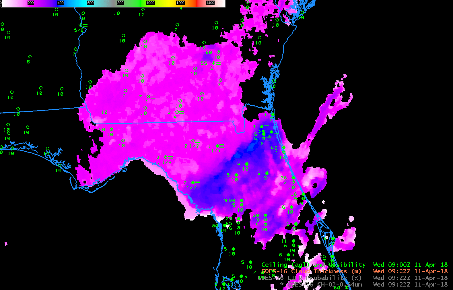
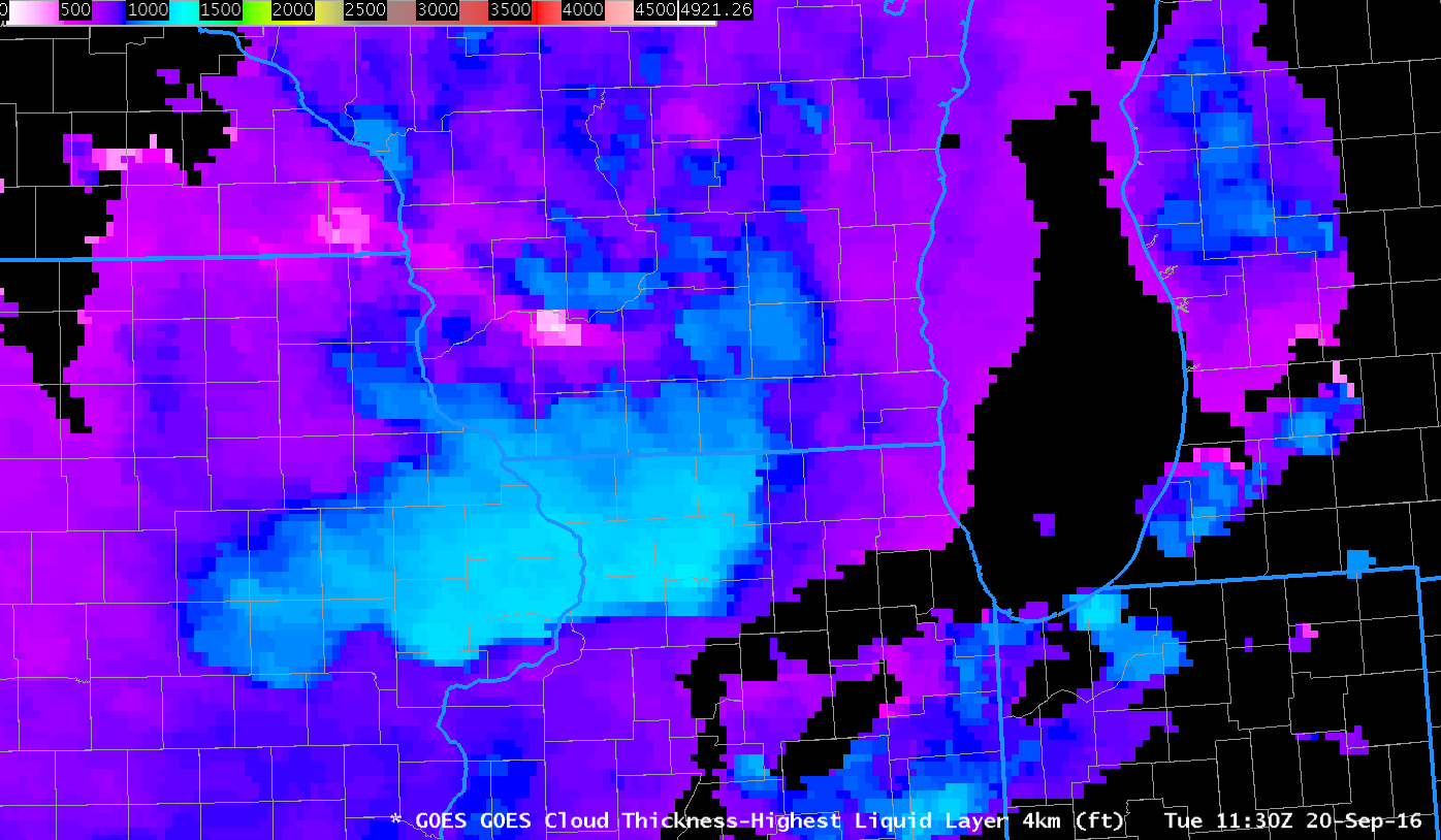
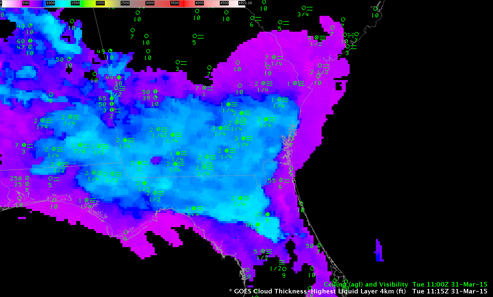
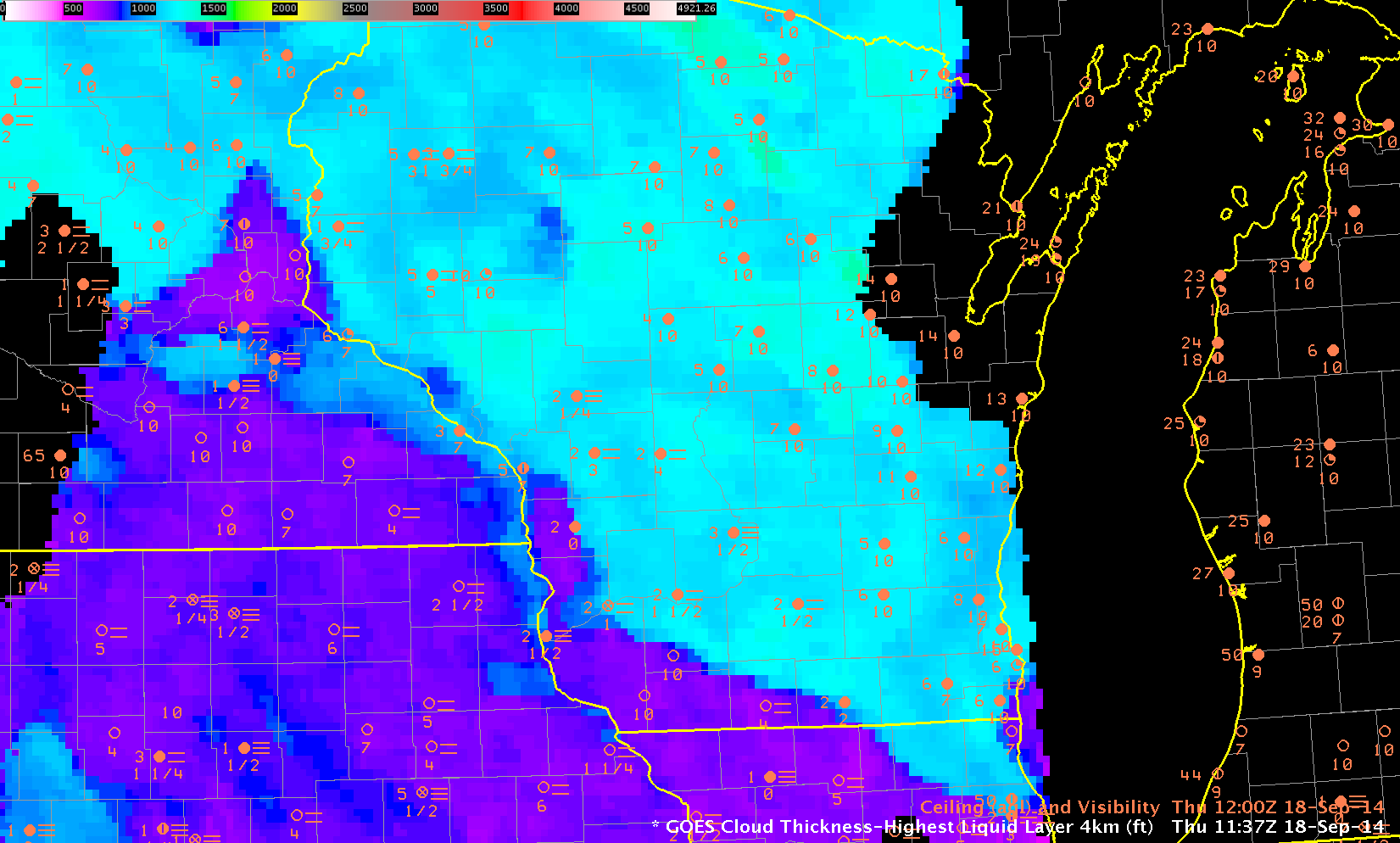
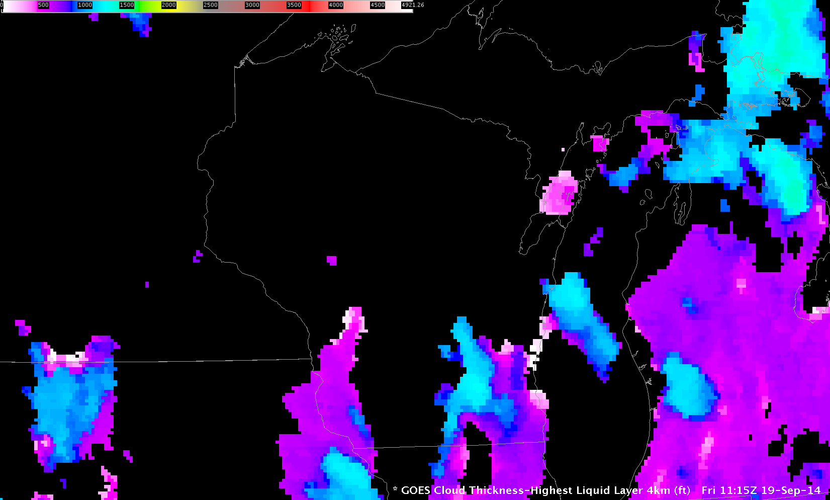
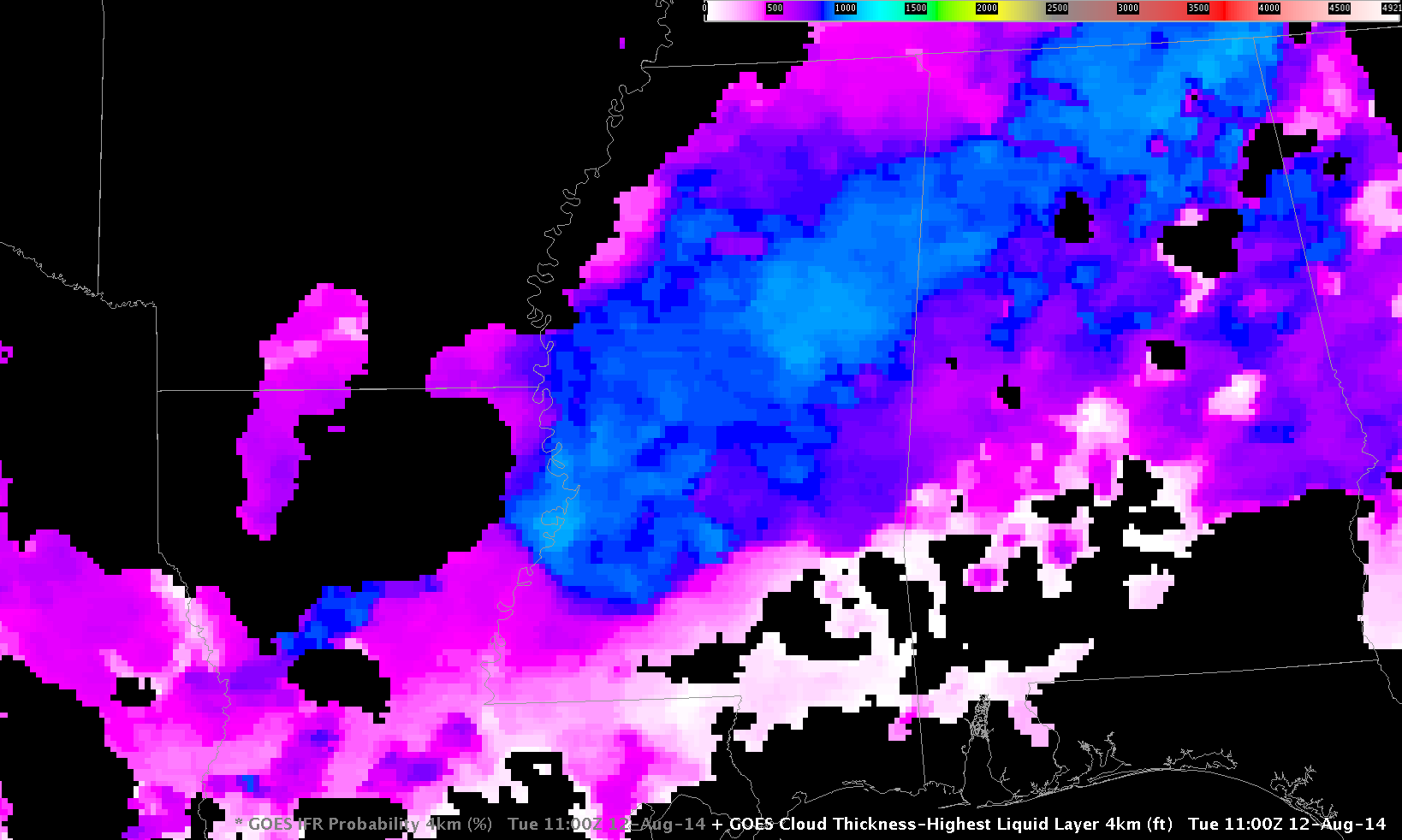
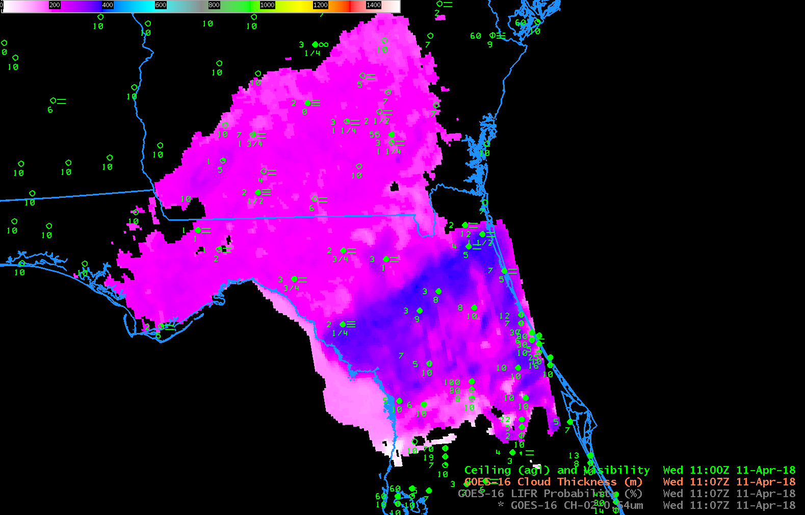
GOES-R Cloud Thickness, 0922-1107 UTC on 11 April 2018 (Click to enlarge)

GOES-R Cloud Thickness can be used (along with this scatterplot) to estimate when fog or low clouds in a region will burn off. This look-up table is most appropriate when used with Radiation Fogs. GOES-R Cloud Thickness is created from a look-up table that was developed using SODAR observations of low clouds off the west coast of the USA and GOES-West (Legacy GOES) observations of 3.9 µm emissivity. These thickness values just before sunrise were then compared to subsequent imagery to determine when the observed fog/low clouds dissipated and the scatterplot was created.

In the case above, the final GOES-R Cloud Thickness field before sunrise conditions occurred at 1107 UTC (Note in the image how low clouds have vanished just off the coast of northeast Florida)   Values over southern Georgia and most of northeast Florida were in the 200-m range:  Very thin!  The scatterplot suggests that such a thickness (equal to about 700 m) will dissipate within an hour. A small strip of somewhat thicker clouds (blue enhancement, suggesting a thickness of 350-400 m) stretched southwestward from Jacksonville to the Gulf of Mexico.

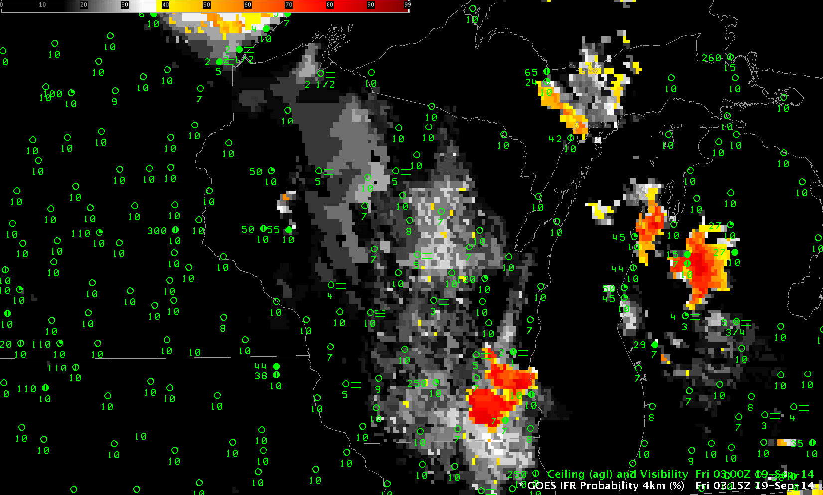
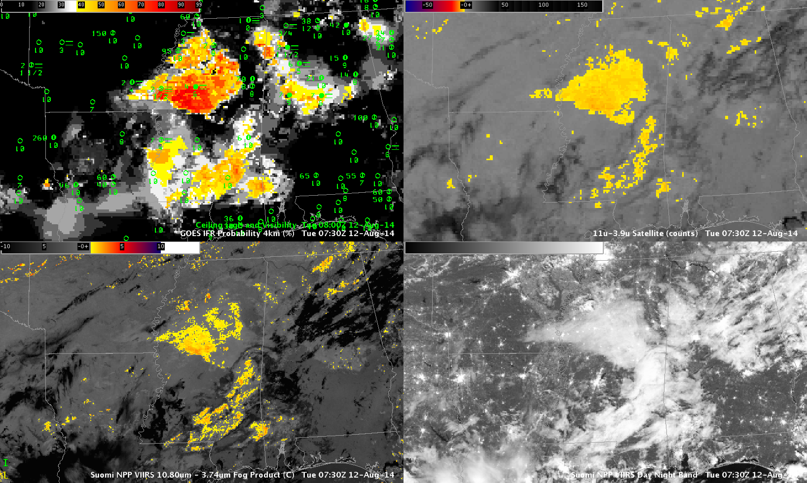
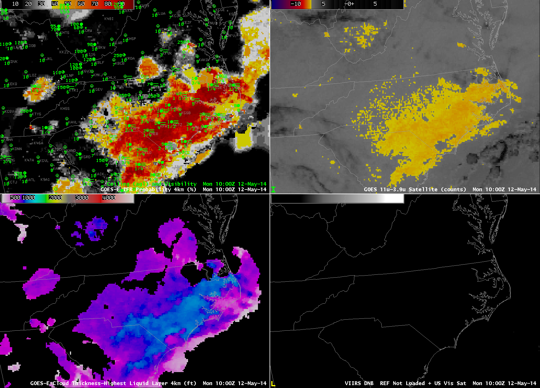
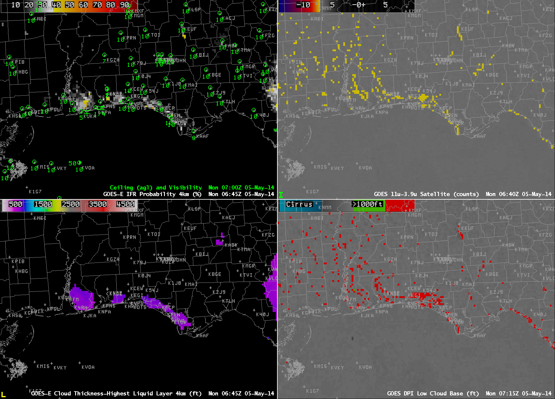
IFR Probabilities during this time before sunrise show enhanced values where IFR and near-IFR conditions are present.  Note that that region of thicker clouds (thicker as diagnosed by the GOES-R Cloud Thickness product) shows higher IFR Probabilities.

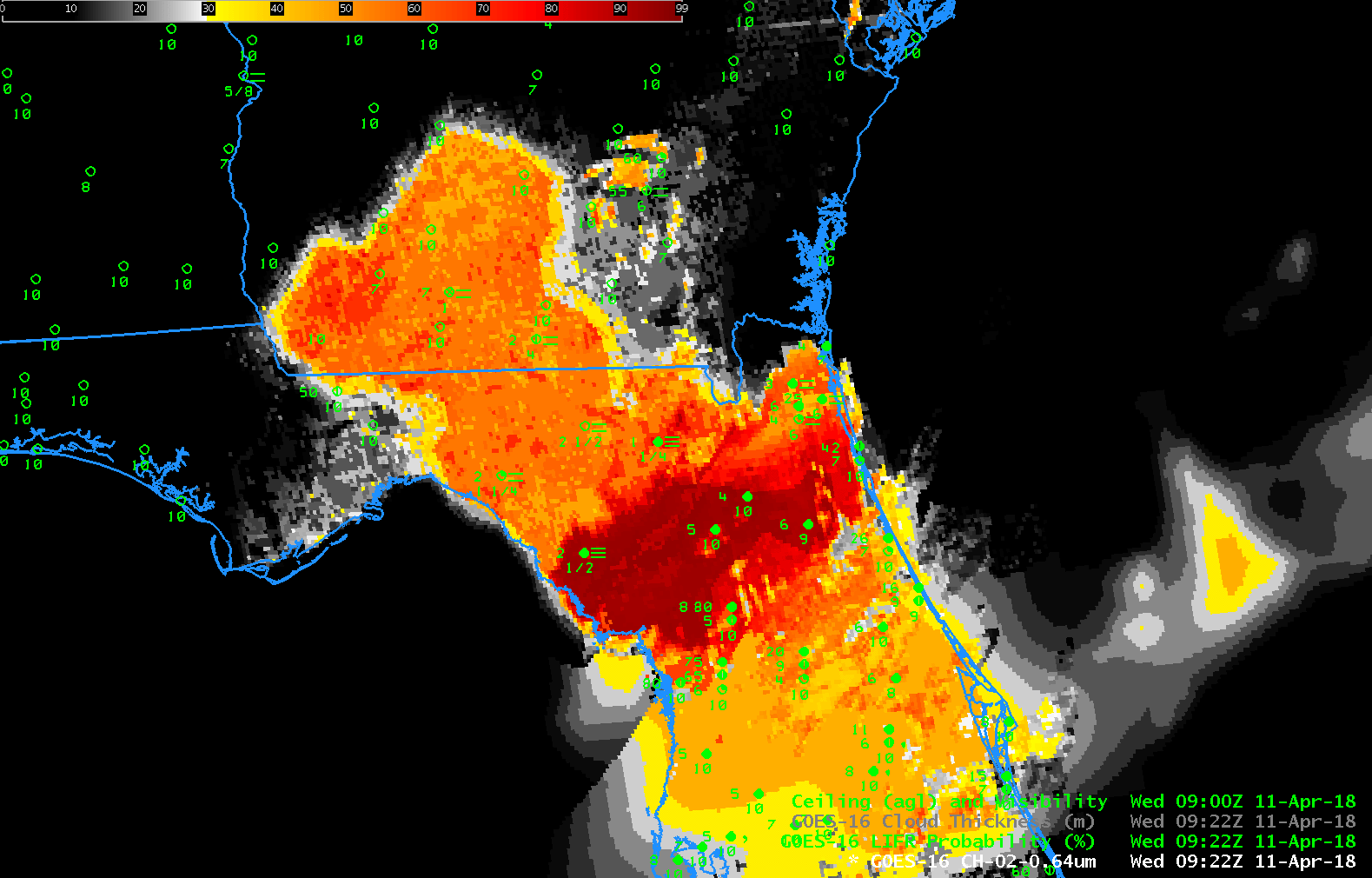
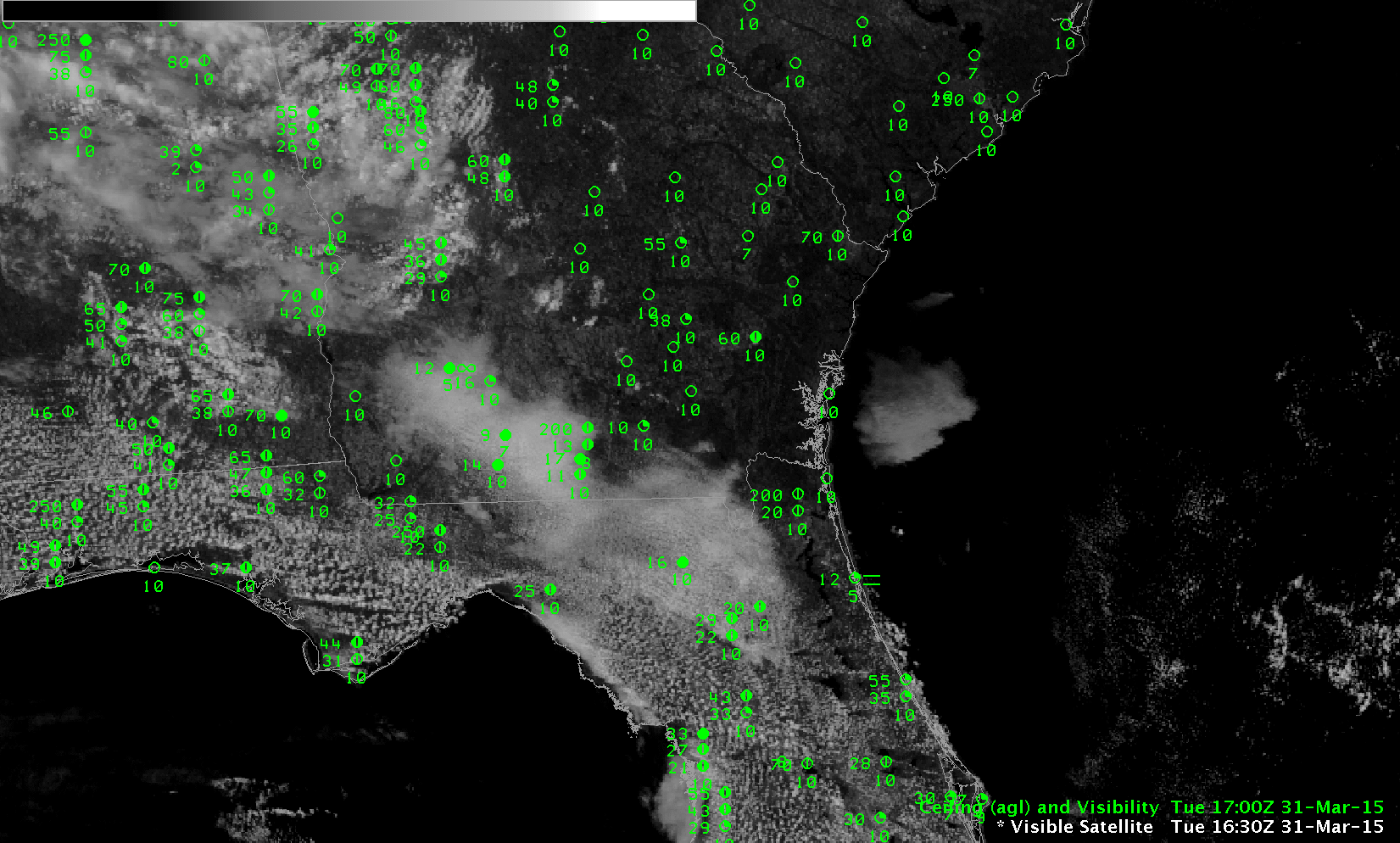
GOES-16 IFR Probabilities, 0922 UTC to 1412 UTC on 11 April 2018 (Click to enlarge)

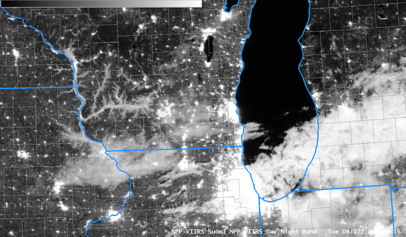
The GOES-16 ‘Night Fog’ Brightness Temperature Difference product, below, shows a small signal over southern Georgia where IFR Conditions are present, and where Cloud Thickness is small.  There is a stronger signal southwest of Jacksonville, which may be one reason that the IFR Probability value there are somewhat stronger than over southern Georgia and extreme northern Florida.  Note also : (1) the sign of the Brightness Temperature Difference flips when the sun rises as increasing amounts of reflected solar 3.9 µm radiation overwhelm the emissivity-driven differences and (2)  the Brightness Temperature Difference field gives little surface information under the cirrus shield over central Florida (or over the Atlantic Ocean).

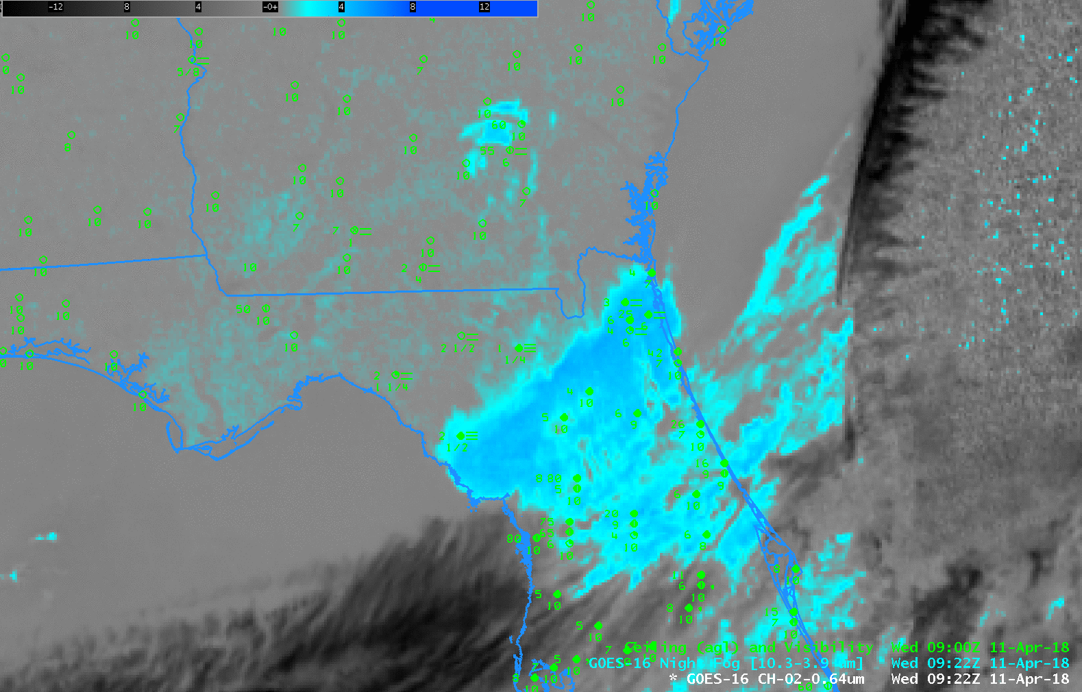
GOES-16 ‘Night Fog’ Brightness Temperature Difference (10.3 µm – 3.9 µm) from 0922 through 1412 UTC on 11 April 2018 (Click to enlarge)

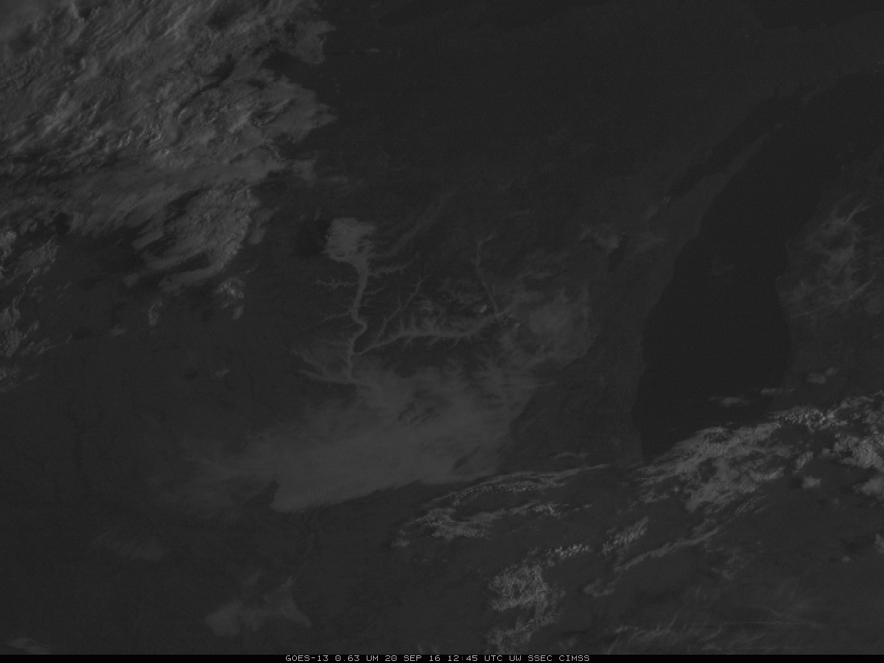
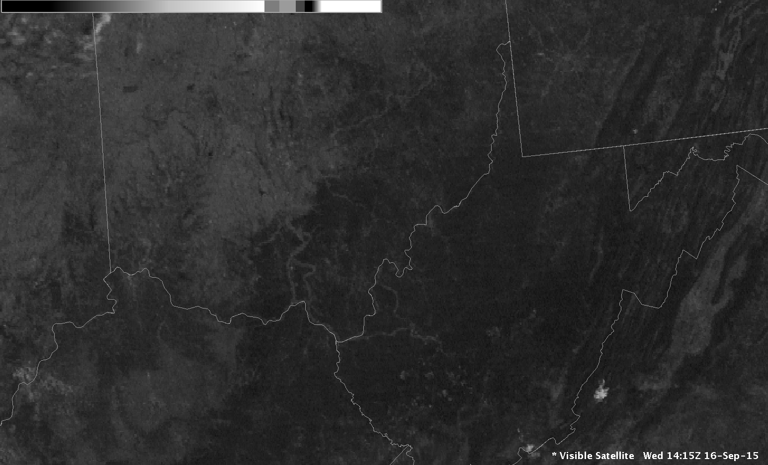
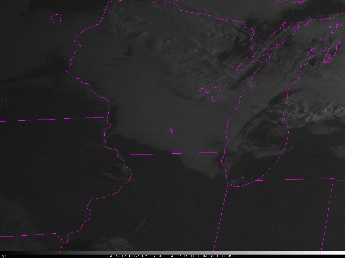
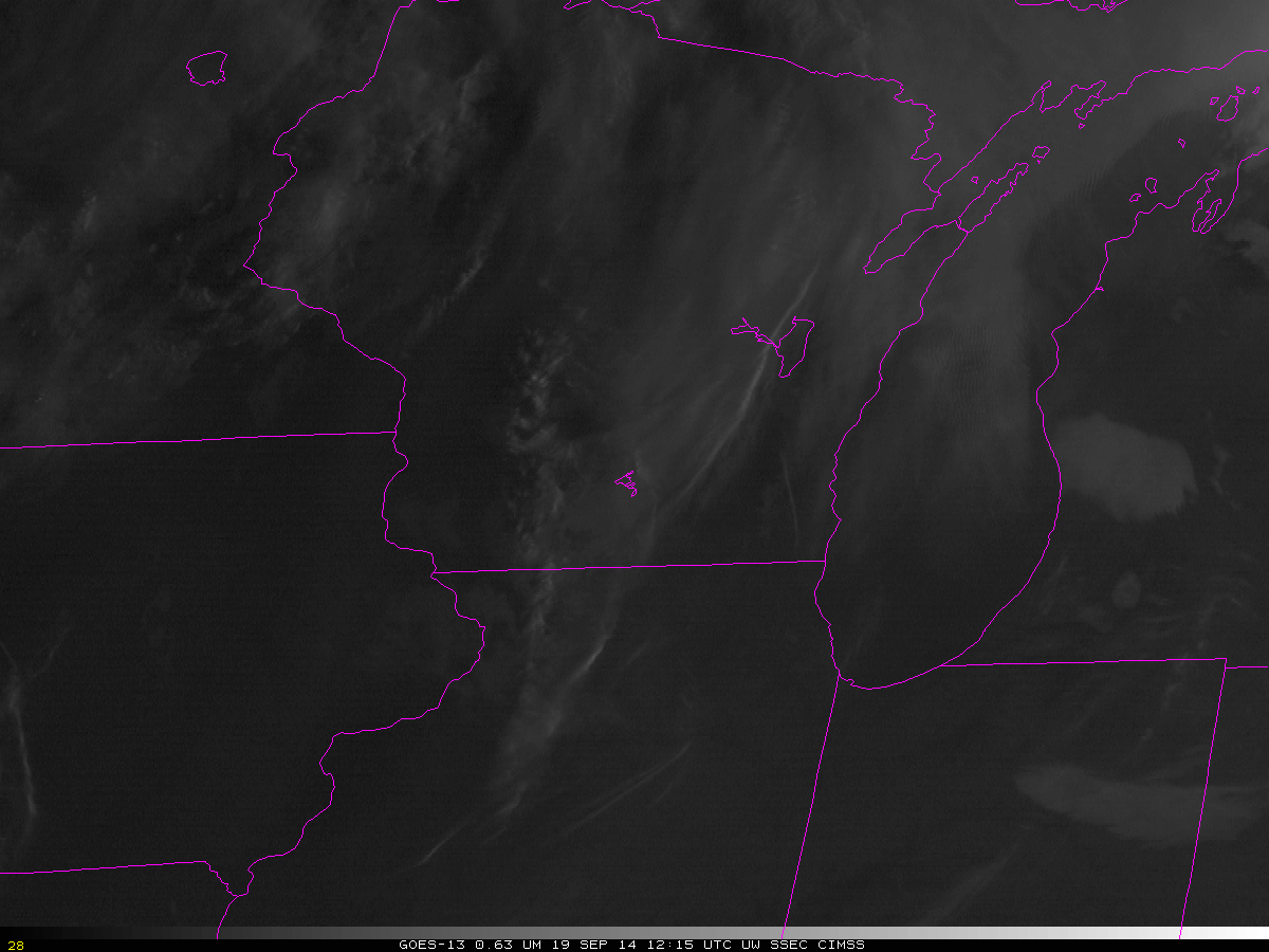
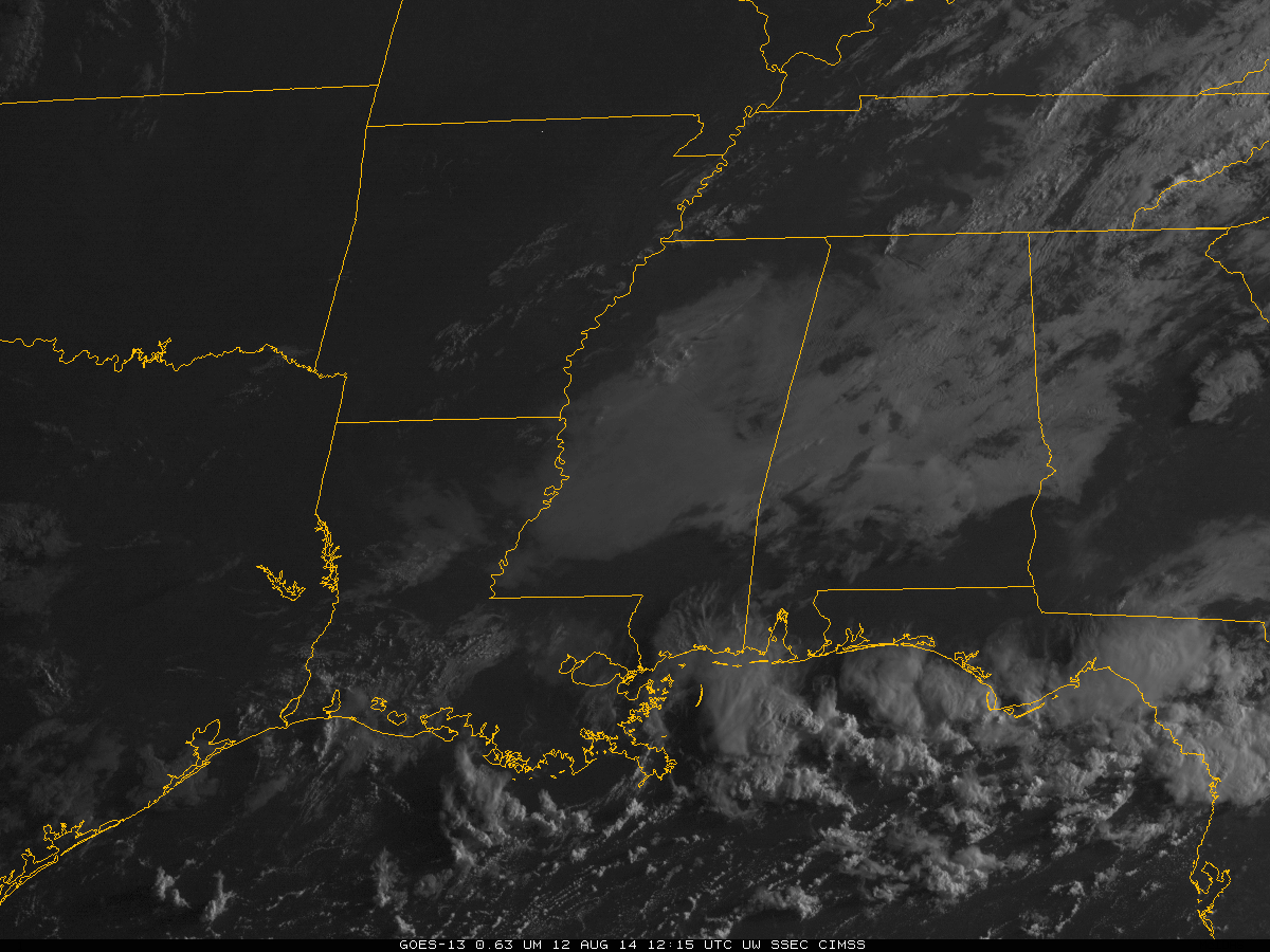
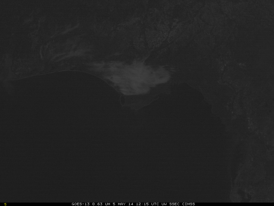
Visible imagery, below, shows a quick dissipation to the fog and low clouds as expected given their diagnosed thin nature by the Cloud Thickness product.

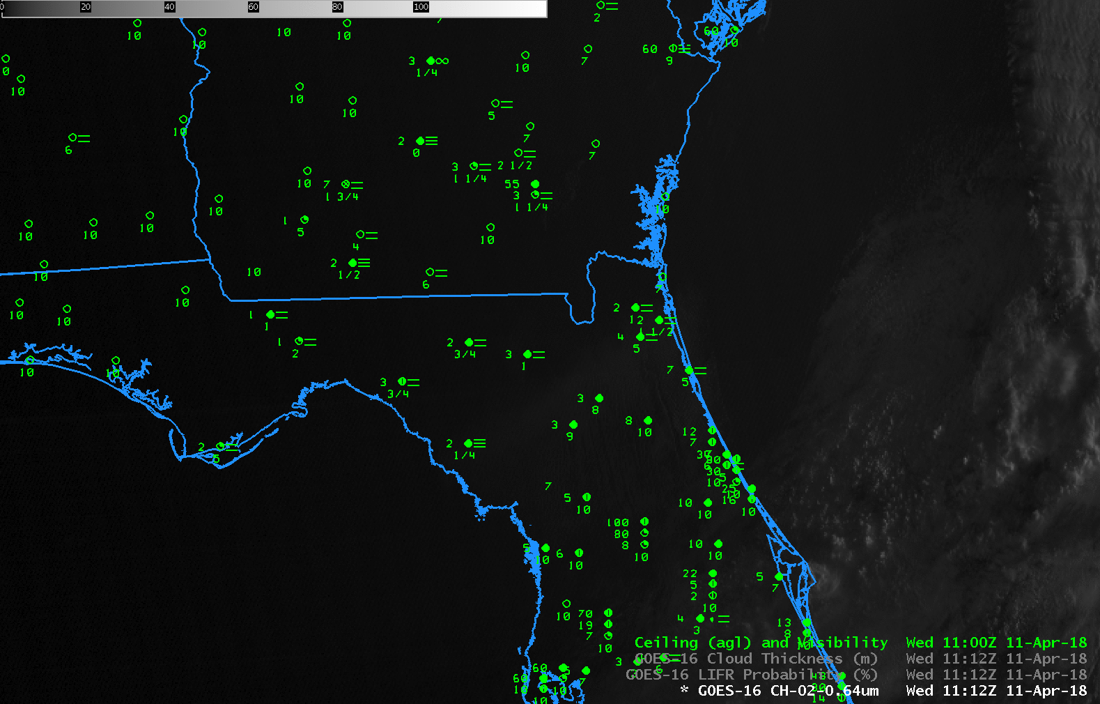
GOES-16 ABI Visible (0.64 µm) imagery, 1112-1412 UTC on 11 April 2018 (Click to enlarge)

Cloud Thickness and Dissipation Time

goes-rcloudthickness_1130utc_20sept2016

GOES-R Cloud Thickness Fields, 1130 UTC on 20 September 2016 (Click to enlarge)

GOES-R Cloud Thickness is created from a look-up table created from observations of 3.9 µm emissivity and sodar observations of cloud thickness off the west coast of the United States.  The product is not computed during twilight conditions when rapid changes in reflected solar radiation (either increases around sunrise or decreases around sunset).  The image above shows the GOES-R Cloud Thickness field over the midwest just before sunrise on 20 September 2016 (Radiation fog formed subsequent to late-afternoon and evening thunderstorms over Wisconsin and Illinois).  This scatterplot relates the last pre-sunrise value to dissipation time.  GOES-R Cloud thickness shows values over the Wisconsin River Valley in southwest Wisconsin, and over regions south of Military Ridge. Largest values — 1100 feet over Illinois and Iowa — suggest (from the scatterplot) a dissipation time of around 4 hours, which would be 1130 UTC (the time of the image) + 4 hours, or 1530 UTC.  There is also a region of thick clouds on northwest Indiana on the shore of Lake Michigan.  It’s these regions where you should expect large-scale fog/low clouds to dissipate last.   The animation below shows that to be true.  Fog over the river valleys is taking a bit longer to dissipate than expected, however. Note: navigation in the animation shows the effect of the loss of one star-tracker on GOES-13.

goes13_flswi_20sept2016_1245_1515anim

GOES-13 Visible (0.63 µm) animation, 1245-1515 UTC on 20 September 2016 (Click to enlarge)

The Day Night band on the VIIRS instrument on board Suomi NPP produces visible imagery at night that showed the regions of fog distinctly shortly after 0800 UTC on 20 September as shown below.

daynightband_wi_0827_20sep2016

VIIRS Day/Night Band Visible (0.70 µm) Imagery from Suomi NPP at 0827 UTC on 20 September (Click to enlarge)

Radiation Fog over South Carolina

goesr_ifrp_13sept2016anim_0200_1000

GOES-R IFR Probability Fields and surface reports of ceilings and visibilities, 0100-1000 UTC on 13 September 2016 (Click to enlarge)

High Pressure over the eastern United States allowed Radiation Fog to form over much of the southeast early on the morning of 13 September 2016.  The GOES-R IFR Probability hourly animation, above, shows increasing probabilities of IFR conditions over much of North and South Carolina, with IFR conditions observed at many stations by sunrise (graphic from here).  IFR Probabilities provided an earlier alert to the fog development (as such, it’s a good situational awareness tool) than was possible from the traditional brightness temperature difference field (see the 0400 UTC image below — click here for a much larger image) because of multiple cloud layers present over the Carolinas in the wake of departing showers. The enhancement for the brightness temperature difference field is such that clouds composed of water droplets are typically shaded orange or yellow.  In the 0400 UTC brightness temperature difference field below (right), fog is not indicated over South Carolina.

tifrp_btd_0400_13sept

GOES-R IFR Probability fields (left) and GOES-13 Brightness Temperature Difference Fields (right), both from 0400 UTC on 13 September 2016 (Click to enlarge)

GOES-R Cloud Thickness fields can be used to estimate fog dissipation time for radiation fog. This scatterplot shows a rough relationship between the last thickness field produced before twilight conditions and the dissipation time. That field is shown below — note that portions of eastern North Carolina have slipped into twilight conditions already by 1100 UTC. Maximum values over South Carolina are around 850 feet (near Greenville/Spartanburg), while those over North Carolina exceed 1200 (near Asheville). Fog dissipation should occur first over South Carolina, then over North Carolina.

goes_r_cloudthickness_1100_13sept

GOES-R Cloud Thickness Field, 1100 UTC on 13 September 2016 (Click to enlarge)

Cloud Thickness and Dissipation Time

Slide136

Dissipation time as a function of GOES-R Cloud Thickness

The chart above shows the relationship between the last pre-sunrise GOES-R Cloud Thickness product and Fog Dissipation time.  Observations of the last pre-sunrise GOES-R Cloud Thickness (developed from an empirical relationship between 3.9 µm emissivity and sodar-observed cloud thickness of the west coast of the USA) can be related to the dissipation time relative to the last observation of Cloud Thickness.  The scatterplot was developed using data mostly over the southeastern part of the USA, but also over the Great Plains.  However, it does have value in other geographic regions too, as shown below.

GOESR_CLDTHICK_IFRPROB_1100UTC_16sep2015toggle

GOES-R IFR Probabilities and GOES-R Cloud Thickness, 1100 UTC 16 September 2015 (Click to enlarge)

On 16 September, river fog developed over the Ohio River and its tributaries in Ohio, West Virginia and Pennsylvania. The toggle above shows GOES-R IFR Probability and GOES-R Cloud Thickness fields at 1100 UTC on 16 September.  This was the last pre-sunrise GOES-R Cloud Thickness over West Virginia (Indeed, the leading edge of twilight — where GOES-R Cloud Thickness is not computed — is apparent at the extreme eastern edge of the image, from Virginia up into central Pennsylvania). The GOES-R Cloud Thickness fields show largest values — around 800 feet — in/around the Ohio River between West Virginia and Ohio. The chart above suggest rapid dissipation. The best fit line (blue) suggests dissipation in about an hour, although there is considerable spread to the values, from 30 minutes up to almost 2-1/2 hours.

Almost two hours later (1245 UTC), fog is still present in isolated patches near the river, and GOES-R IFR Probability fields are suggesting fog is still present as well.  The horizontal extent of the GOES-R IFR Probability field is greatly reduced because visible imagery can be used after sunrise to screen out clear regions (Cloud-clearing in the algorithm is more effective).  By 1415 UTC (bottom), three hours after the GOES-R Cloud Thickness imagery above, all fog has evaporated.

GOES_VIS_GOESRIFRPROB_1245UTC_16sep2015toggle

GOES-R IFR Probabilities and GOES-13 Visible Imagery (with a low-light enhancement), 1245 UTC 16 September 2015 (Click to enlarge)

GOES_VIS_1415UTC_16sep2015

GOES-13 Visible Imagery, 1415 UTC 16 September 2015 (Click to enlarge)

Dissipation Time

CloudThickness_1115_31March2015

GOES-R Cloud Thickness over southern Georgia/northern Florida, 1115 UTC on 31 March 2015 (Click to enlarge)

If fog has formed via radiational cooling, the GOES-R Cloud Thickness product that is produced just before sunrise can be used to estimate when clouds will clear. Such an image is shown above for a case of dense fog over southern Georgia on 31 March 2015. The largest Cloud Thicknesses at this time were around 1150 feet over the southern part of this region. Based on this correlation curve, then, dissipation where the fog is thickest should occur 4-1/2 to 5 hours after 1115 UTC. The visible animation below suggests that dissipation was complete by 1715 UTC.

VIS_1630to1730_31March2015

Visible Imagery, 1630-1815 UTC on 31 March 2015 (Click to enlarge)


Cloud Thickness as a Predictor of Fog Dissipation, part II

This post showed examples of Cloud Thickness and how its use as a predictor for dissipation time might be incorrect because of synoptic or mesoscale forcing.

Radiation fog formed in River Valleys of Wisconsin early in the morning on 22 September, and the image below shows the final Cloud Thickness field computed before twilight conditions developed over western Wisconsin (twilight conditions are already occurring over eastern Wisconsin).

CloudThickness_1145UTC_22Sep2014

GOES-R Cloud Thickness (of the highest liquid water cloud layer) just before sunrise, 22 September 2014

Cloud Thickness values near LaCrosse, WI, are around 900 feet; values are closer to 1200 feet over northeast Wisconsin along the St. Croix River. The chart suggests a dissipation time over the southwest part of Wisconsin of around 3 hours, and more than 4 hours over northwestern Wisconsin. The animation below shows that those estimates were accurate.

GOES13_VIS_22Sept_1215-1515

GOES-13 Visible (0.63 µm) Animation over Wisconsin, 22 September, 1215-1515 UTC (Click to animate)

Cloud Thickness as a Predictor of Fog Dissipation

GOES_R_Cloud_Thickness_1137UTC_18Sep2014

GOES-R Cloud Thickness over Wisconsin and surrounding States, 18 September 2014, just before sunrise (Click to enlarge)

GOES-R Cloud Thickness can be used as a predictor for dissipation time of Radiation Fog, using this chart and the thickness (as above) from the last pre-dawn GOES-R Cloud Thickness field (Recall that GOES-R Cloud Thickness is not computed in the few hours of twilight surrounding sunrise or sunset; in the image above, twilight has reached lower Michigan but not yet Wisconsin). However, it’s important to remember that the chart is valid for radiation fog. Other forcings might cause fog to dissipate (or persist).

In the example above, Cloud Thickness values ranges from around 700 over southwest Wisconsin to as much as 1400 over north-central Wisconsin. Most of south-central Wisconsin (cyan) has values around 1200. According to the best-fit line, that suggests a burn-off time of more than 5 hours (although those values are extrapolated; note that no values that large went into the creation of the best-fit line) over WI, except over southwestern WI where a burn-off time of less than 1 hour is predicted. Did that work out?

The animation below shows fog/low stratus moving towards the southwest with time. The cool and damp northeasterly flow from the Great Lakes into Wisconsin (surface map at 1800 UTC on 18 September) suppressed the heating necessary to reduce the relative humidity and foster fog evaporation. Perhaps the fog initially formed as advection fog; however, the northeasterly flow that developed early in the morning on 18 September came from a synoptic set-up that allowed fog to persist longer than the GOES-R Cloud Thickness algorithm suggests. This is not an uncommon occurrence. Clouds did not burn off over south-central WI until after 1800 UTC. During September, delayed burn-off of morning clouds can significantly affect the day-time temperature.

WIFOG_18Sep2014_12-20loop

Half-hourly visible imagery over Wisconsin, 1215-2045 UTC on 18 September (Click to animate)

=============================================================================

Low clouds and fog redeveloped during the morning of the 19th of September as well. This occurred during persistent southerly flow in advance of a low pressure system over the Northern Plains. The hourly animation of IFR Probabilities, below, shows IFR Probabilities developing over the course of the early morning of the 19th between 0315 and 1215 UTC. The animation shows a gradual overspreading of the IFR Probability field with higher clouds moving in from the west. (Here is a toggle between IFR Probability and GOES-13 Brightness Temperature Difference Fields at 1115 UTC; note how smooth the field is over much of WI where only Rapid Refresh model data can be used in the computation of the IFR Probability).

GOESR_IFRPROB_WI_19Sep2014_03-12

GOES-R IFR Probability fields, hourly from 0315-1215 UTC on 19 September (Click to animate)

When high clouds overspread the scene, GOES-R Cloud Thickness is not computed. Thus, the last image before twilight, below, shows Cloud Thickness in only a few locations, but those values over southeast Wisconsin exceed 1200 feet, suggesting a burn-off of around 1615 UTC — 5 hours after this last Cloud Thickness image. In this case, that is an overestimate because the southerly winds over WI promote mixing, and the fog quickly dissipates after sunrise. It’s important to consider the synoptic forcing when you use Cloud Thickness. The last Cloud Thickness field and its use as a predictor for fog dissipation (using this chart) is most useful for radiation fog. The visible imagery animation at the bottom shows that the fog dissipated by 1415 UTC.

GOESR_CTH_WI_19Sept2014-9

GOES-R Cloud Thickness just before Sunrise (1115 UTC on 19 September 2015) (Click to enlarge)

WIFOG_19Sep2014_12-16loop

GOES-13 Visible Imagery, 1215-1615 UTC on 19 September (Click to animate)

Fog over Mississippi

FourPanel_0730UTC_12August2014

GOES-R IFR Probabilities computed from GOES-13 at 0730 UTC (Upper Left), GOES-13 Brightness Temperature DIfference (10.7 µm – 3.9 µm) (Upper Right), Suomi NPP VIIRS Brightness Temperature Difference (11.35 µm – 3.74 µm) (Lower Left), Suomi NPP VIIRS Day Night Band (Lower Right), all at 0730 UTC on 12 August 2014

Fog developed overnight in central Mississippi, and the imagery above, at 0730 UTC, is a snapshot during the development. The just-past-full moon provided plenty of illumination, so the stratus and cirrus clouds over the south are distinct. It can be difficult, however, using only the Day Night Band to distinguish between low stratus (north-central Mississippi), mid-level stratus (eastern Mississippi), and high, thick cirrus (Alabama). In addition, the Day Night Band and the brightness temperature difference fields give information at the top of the cloud only. Information about the bottom of the cloud — whether the stratus deck extends to the surface as fog, for example, is difficult to glean from cloud-top properties. This is where the IFR Probability field that incorporates both cloud-top features derived from the brightness temperature difference field and lower-tropospheric information extracted from the Rapid Refresh Model can improve the detection of reduced ceilings and visibilities. Suomi NPP and other polar orbiters can give high spatial resolution imagery. GOES data has excellent temporal resolution to monitor how things evolve with time. The animation below shows how the fog/low stratus developed over the course of the day.

GOES_IFR_Prob_12August2014loop

GOES-R IFR Probabilities and Surface observations of visibility/ceilings, hourly 0200-1100 UTC 12 August 2014

The fields in the animation above change character over the course of the night. Initially, the fields over southwestern Mississippi are very smooth; in this region, multiple cloud layers (a thunderstorm complex was dissipating) prevent any satellite signal from being used as a predictor for IFR Probabilities; only model data are being used. As the night progresses and the mid-level and upper-level clouds dissipate, the character of the field takes on a more pixelated appearance that means satellite data are being used as a predictor. The addition of satellite data to the suite of predictors also means that the probability value increases. By the end of the night, high probabilities have overspread much of central Mississippi, and low ceilings and reduced visibilities are widespread.

GOES-R Cloud Thickness can be used to estimate times of fog dissipation, using the relationship in this scatterplot and the Cloud Thickness in the last pre-sunrise scene, shown below for 12 August 2014. The thickest values are near Vicksburg, MS, where GOES-R Cloud Thickness approaches 1000 feet.  That suggests a clearing time around 1400 UTC, ~3 hours after the valid time of the image below.  The visible animation of the low clouds clearing is below.

CloudThickness_11UTC_12August2014

GOES-R Cloud Thickness, 1100 UTC 12 August 2014

GOES13_KJAN_VIS_12August2014loop

Radiation fog over coastal North Carolina

GOES_IFR_PROB_20140512_1000

GOES-R IFR Probabilities with observations of ceilings/visibilities (Upper Left), GOES-East Brightness Temperature Difference (10.7µm – 3.9µm) (Upper Right), GOES-R Cloud Thickness (Lower Left), Suomi/NPP VIIRS Day/Night Band (0.70 µm, at night) or GOES-East Visible imagery (0.63 µm, during day), Times as indicated (Click to enlarge)

Clear skies allowed for radiation fog with IFR conditions to develop over eastern North Carolina overnight. GOES-R Cloud Thickness as observed at the last time before twilight conditions begin — in this case at 1000 UTC (6 AM EDT) — can be used as a predictor for fog dissipation time using this chart. At 1000 UTC, maximum cloud thickness was 1000 feet, which suggests a dissipation time around 1300-1330 UTC.

The visible animation, below, is in agreement with the prediction from the cloud thickness field.

GOES13_VIS_NC_loop_12MAY2014

GOES-East Visible Imagery (0.62 µm) Times as indicated (Click to enlarge)

A toggle of two images with Day/Night band imagery, below, shows the difficulty in using the Day/Night band to identify regions of fog/low clouds consistently. In the 0615 UTC image, the developing low clouds show up well (Of course, it’s hard to tell if the clouds are low stratus or mid-level stratus), but the picture at 0745 UTC is a lot less distinct.

GOES_IFR_PROB_20140512_toggle_0615_0745

GOES-R IFR Probabilities with observations of ceilings/visibilities (Upper Left), GOES-East Brightness Temperature Difference (10.7µm – 3.9µm) (Upper Right), GOES-R Cloud Thickness (Lower Left), Suomi/NPP VIIRS Day/Night Band (0.70 µm), Times as indicated (Click to enlarge)

A toggle of two images with Day/Night band imagery, below, shows the difficulty in using the Day/Night band to identify regions of fog/low clouds consistently. In the 0615 UTC image, the developing low clouds show up well (Of course, it’s hard to tell if the clouds are low stratus or mid-level stratus), but the picture at 0745 UTC is a lot less distinct.

Radiation Fog in the Florida Panhandle

GOES_IFR_PROB_20140505loop

GOES-R IFR Probabilities computed from GOES-East (Upper Left), GOES-East Brightness Temperature Difference (10.7 µm – 3.9 µm) (Upper right), GOES-R Cloud Thickness (Lower Left), GOES-13 Heritage Cloud Thickness Product (Lower Right), times as indicated (Click to enlarge)

Clear skies and light winds over the Florida Panhandle allowed radiation fog to develop, and the GOES-R IFR Probability field ably captured the region of IFR conditions, as shown above. Note how the GOES-R Fields provide information that looks less ‘noisy’: the heritage products — Brightness Temperature Difference and Cloud Thickness — both have signals over interior Alabama and Mississippi where IFR conditions were not reported. In addition, the well-known co-registration error in the 10.7 and 3.9 sensors produces a faulty signal along the Florida coast east of Appalachee Bay. Eventually this signal because so strong that it bleeds into the GOES-R IFR probability.

Cloud thickness can be used to forecast fog dissipation time, using this chart and tempered by experience. The last pre-sunrise cloud thickness is shown at 1045 UTC in the loop above, and is around 1000 feet, suggesting a dissipation time around 1345 UTC. The visible animation below corroborates this estimate.

GOES13_FL_FOG_5MAY2014loop

GOES-R Visible (0.63 µm), times as indicated (Click to enlarge)