Category Archives: Multiple Cloud Layers

How to tell at a glance that IFR Probability is model-driven: Pacific Northwest version

GOES-16 IFR Probability at 10-minute timesteps, 1051 to 1721 UTC on 6 February 2020 (Right click to enlarge)

The animation above, of GOES-16 IFR Probability, shows high IFR values in regions over western Washington and Oregon, and those high values correlate spatially very well with surface observations of low ceilings and reduced visibilities.b You will note a couple things in the animation: The field is mostly stationary, with slight adjustments on every hour. Those small changes reflect the change in the model fields (hourly Rapid Refresh) that are used to complement satellite estimates of low clouds in the computation of IFR Probabilities.

On this day, the satellite did not view many low clouds (some are apparent in southwestern Oregon). The flat field (vs. the more pixelated view over southwest OR, and also occasionally in the west-northwest flow coming in off the Pacific) suggests only model data are being used. The stepwise changes on the hour also suggest that.

The animation of the Night Fog Brightness Temperature Difference (10.3 µm – 3.9 µm) field, below, has a signal that is consistent with the lack of observed stratus over the coastal Pacific Northwest. Note also how the Night Fog Brightness temperature difference field flips sign as the Sun comes up and the 3.9 µm signal becomes larger due to reflected solar radiance with a wavelength of 3.9 µm.

GOES-16 Night Fog Brightness Temperature Difference (10.3 µm – 3.9 µm) at 10-minute timesteps, 1051 to 1721 UTC on 6 February 2020 (Right click to enlarge)

GOES-16 views of the Pacific Northwest show fairly large pixel sizes. NOAA/CIMSS scientists have been creating GOES-17 IFR Probability for the past couple weeks, and this product will become available via an LDM field in the near future.

Note that GOES-17 IFR Probability products are available online at https://cimss.ssec.wisc.edu/geocat.

IFR Probability, Brightness Temperature Differences and Nighttime Microphysics RGB estimates of Fog

GOES-16 Brightness Temperature Difference (10.3 µm – 3.9 µm), Nighttime Microphysics RGB and IFR Probability Fields, 1126 UTC on 17 December 2019. Also included are sky conditions, ceilings and visibilities in black or green.

Fog and low clouds were widespread over the eastern half of the United States on 17 December 2019. In this example over ArklLaTex the Brightness Temperature Difference suggests low stratus clouds over the region, and the Nighttime Microphysics shows a signal congruent with low clouds. Note, however, that observations over much of the region do not suggest IFR conditions are present. Accordingly, IFR Probability shows fairly low probabilities in this region, with values increasing to the north where visibilities decrease. IFR Probability fields screen out regions of elevated stratus because the Rapid Refresh model in this region does not suggest low-level saturation. Over northeast Oklahoma and northwest Arkansas, however, saturation at low levels is more likely and IFR Probabilities there are larger.

At the same time, high clouds overspread most of the east coast as a storm moved through the area. The high clouds prevent the satellite from seeing low clouds, so both the Brightness Temperature Difference and the Nighttime Microphysics RGB will not have a signal that comports with low stratus detection. However, IFR Probability includes a signal from the Rapid Refresh model if that model shows low-layer saturation in a region of multiple cloud layers; IFR Probability has a strong signal on this date over the east coast were clouds and fog are widespread. IFR Probability also shows IFR Conditions under the low clouds that the satellite does detect over eastern Ohio, and correctly notes the a region of higher ceilings over West Virginia, western Virginia and eastern Tennessee.

When high clouds are not present, there are different equally good ways to estimate low clouds, and that’s shown above. The Brightness Temperature Difference fields, the Nighttime RGB and the IFR Probability fields all tell a similar tale: Much of Iowa and regions to the south and northeast have low ceilings and reduced visibility.

Careful observers to the toggle note that the RGB has a different color over Wisconsin compared to Iowa. In part this is because the Brightness Temperature Field has values that are smaller over Wisconsin. A bigger driver of the color difference, however, is the 10.3 µm brightness temperature — the blue component of the Nighttime Microphysics RGB. Values are around -25º C over Wisconsin, and closer to -10º C over Iowa!

Nighttime Microphysics RGB and Band 13 10.3 µm Brightness Temperature, 17 December 2019

Fog detection when Cirrus is present: Southern Plains edition

GOES-16 Night Fog Brightness Temperature Difference (10.3 µm – 3.9 µm) at 0906, 1006, 1106, 1206, 1306 and 1401 UTC on 8 November 2019 (Click to enlarge)

Consider the stepped 1-hour images of the ‘Night Fog’ Brightness Temperature Difference (10.3 – 3.9) field, above. (Here’s one with full temporal resolution) Extensive jet stream cirrus is preventing GOES-16 from seeing evidence of low clouds, and the satellite alone is therefore failing to identify regions of low ceiling and fog over much of Texas. (The Nighttime Microphysics RGB that depends on the Night Fog brightness temperature difference to detect low clouds suffers from a similar shortcoming here : link )

When Cirrus covers an area of low clouds, GOES-R IFR Probability does allow for low cloud/fog detection because it incorporates low-level saturation information from the Rapid Refresh to delineate regions of fog. Similarly, it can screen out regions of mid-level stratus that can appear as fog in both the Night Fog brightness temperature difference and the Nighttime Microphysics RGB: Note the region around Childress TX, for example, where IFR Probability is low, but where the Night Fog Brightness Temperature Difference has a strong signal in the presence of elevated stratus. Regions around Midland are highlighted in IFR Probability — Rapid Refresh data there are correctly diagnosing low ceilings and reduced visibilities. (Here’s IFR Probability with an animation at full temporal resolution). Because Rapid Refresh model data input into the IFR Probability computation changes every hour, you will sometimes see a pulsing in the imagery.

Use IFR Probability to detect regions of low ceilings and reduced visibility when cirrus has overspread your area.

GOES-R IFR Probability at 0906, 1006, 1106, 1206, 1306 and 1401 UTC on 8 November 2019 (Click to enlarge)

Fog Detection when Cirrus is present

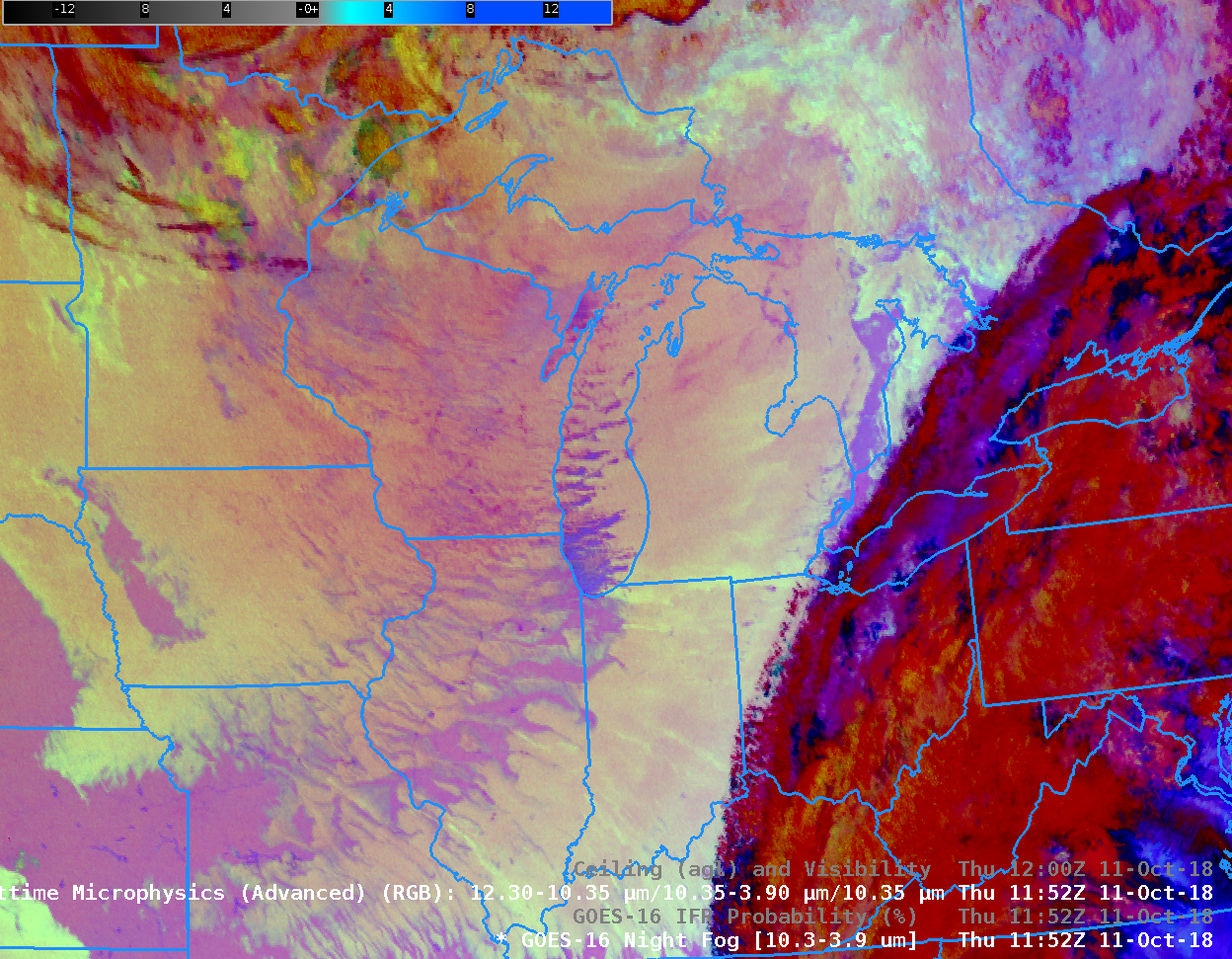
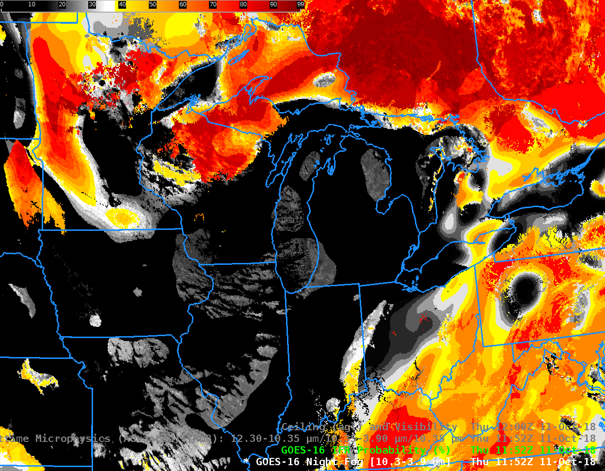
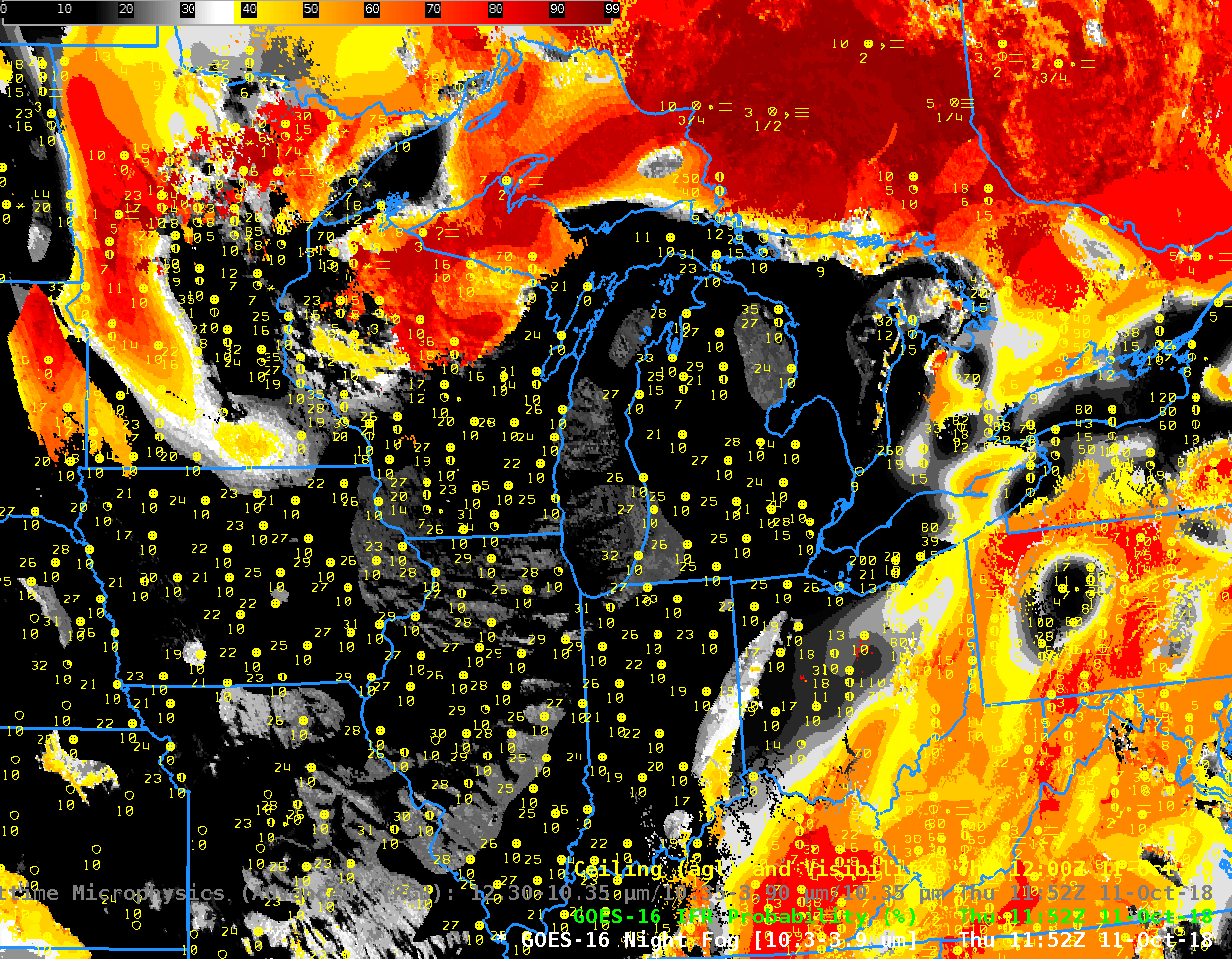
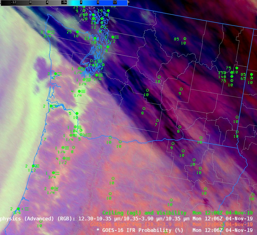
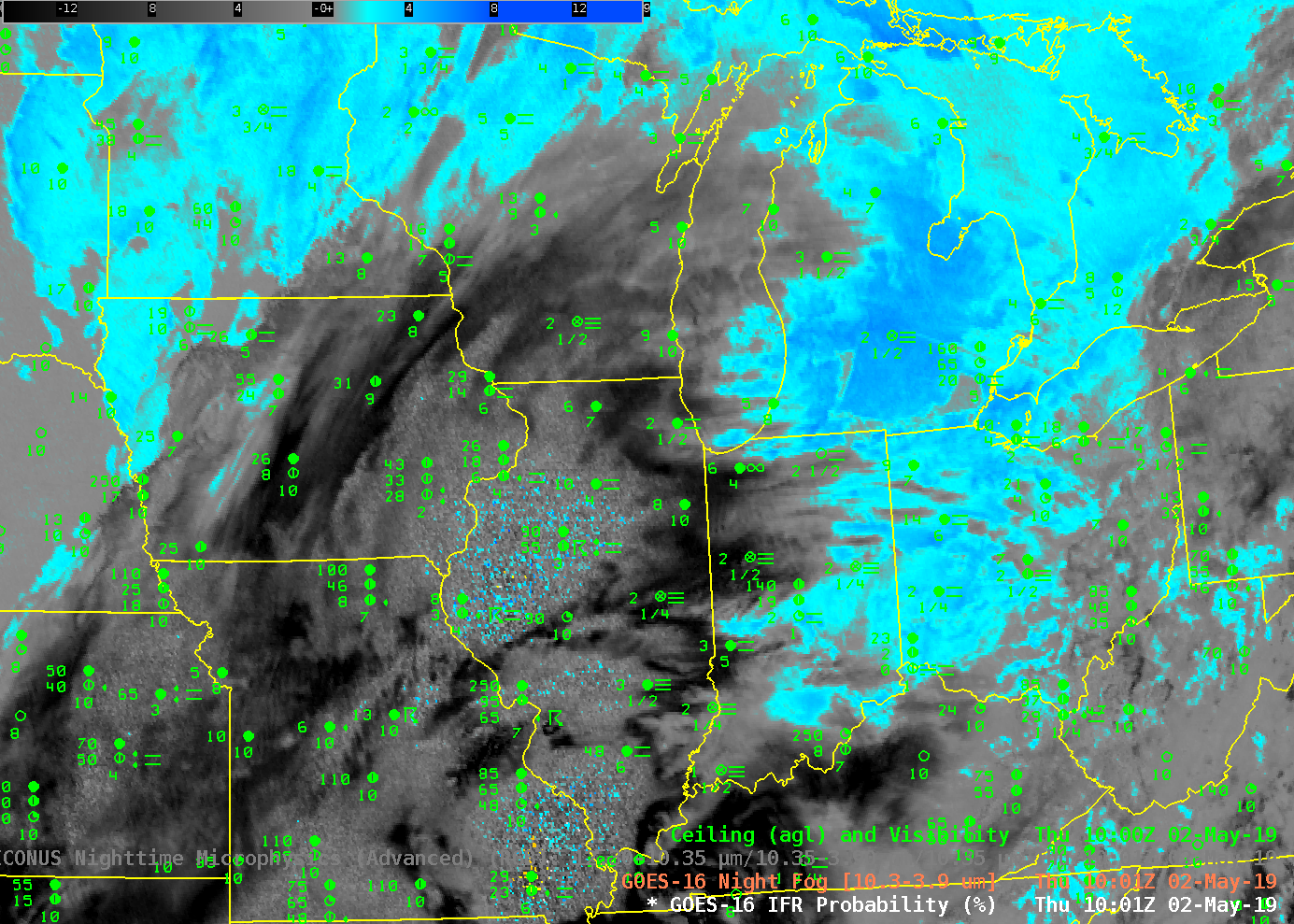
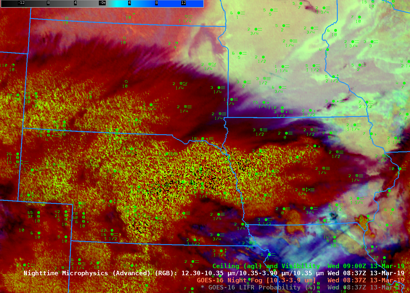
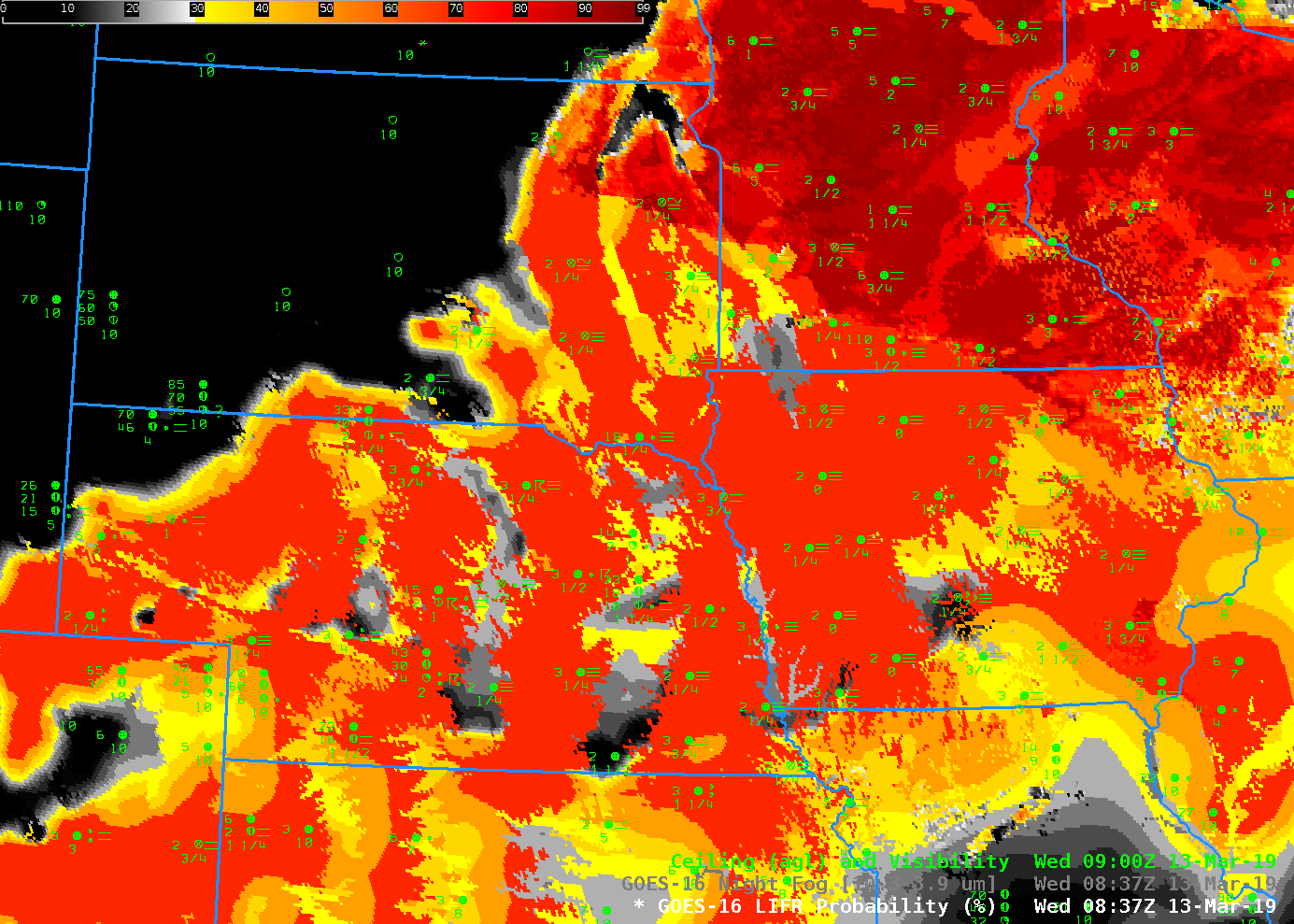
GOES-16 NightTime Microphysics, Night Fog Brightness Temperature Difference (10.3 µm – 3.9 µm) and IFR Probability at 1206 UTC on 4 November 2019, along with 1200 UTC observations of ceilings and visibilities (Click to enlarge)

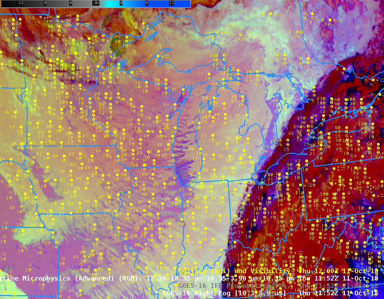
Fog can be a challenge to detect from satellite for two reasons: High clouds can block the satellite’s view of low clouds, or low clouds (stratus) can be detected but the satellite cannot accurately determine the cloud base. The toggle above cycles between the Night Fog Brightness Temperature difference (10.3 µm – 3.9 µm), the Nighttime Microphysics RGB (the Night Fog Brightness Temperature Difference is the green component of that RGB), and GOES-R IFR Probability.

The Night Fog Brightness Temperature Difference can be used to detect low stratus clouds because the small water droplets that make up those clouds have different emissivities at 10.3 µm and 3.9 µm: water droplets do not emit 3.9 µm radiation as a blackbody would, but they do emit 10.3 µm radiation more nearly like a blackbody. Thus the amount of energy at 3.9 µm collected by the satellite is smaller than it would be above a blackbody emitter. The computation of the blackbody temperature associated with the collected energy assumes a blackbody emission. Because that’s not the case at all wavelengths above clouds made of water droplets, 3.9 µm brightness temperatures are colder than those computed from observed 10.3 µm energy.

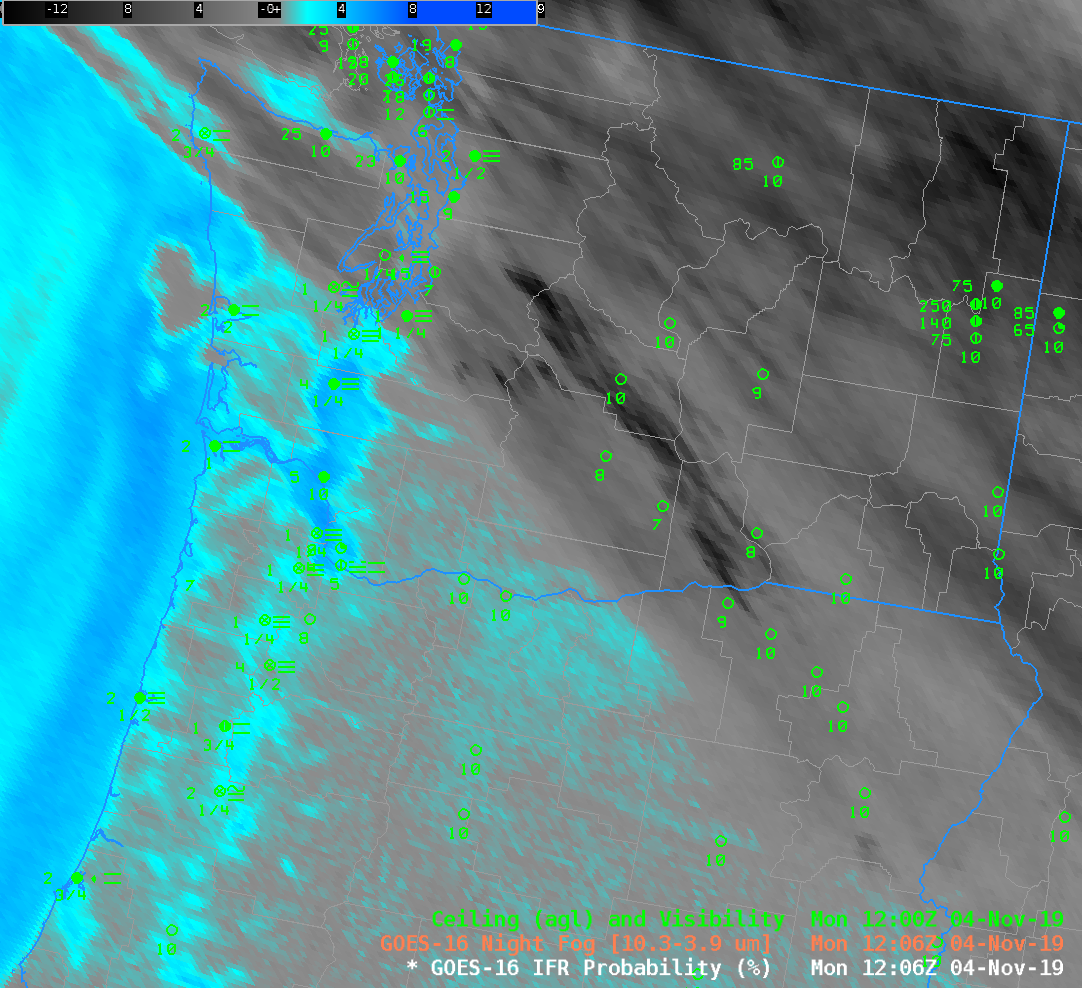
The Night Fog brightness temperature difference field allows an observer to infer the presence of low clouds over the Pacific Ocean, in and around Portland OR on the Columbia River to the ocean, and also northward towards Puget Sound, and in the Willamette Valley between Portland and Eugene OR. There is also a signal over north-central Oregon that is likely unrelated to clouds — variable surface soil emissivity in that region is affecting this brightness temperature difference (The GOES-R Cloud Phase product and Cloud Mask both show no cloud signal in that region).

Note that a cirrus shield is apparent over the northeast half of the image. The cirrus covers most of Puget Sound in Washington, and the Brightness Temperature Difference field can therefore not give information about low clouds (except where breaks in the cirrus occur — such as in the Strait of Juan de Fuca).

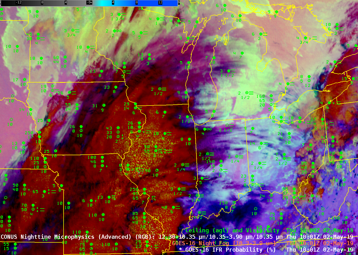
The Nighttime Microphysics RGB is a way to identify low clouds — but its information is coming from the Night Fog brightness temperature difference and it has limitations that are similar to those with the brightness temperature difference, namely: what is going on under cirrus clouds, and how close to the ground are the low clouds that are detected? In the RGB, low clouds will have a yellowish hue (red — the split window difference and green — the night fog brightness temperature difference — make yellow). The RGB shows different values over Portland than over the Willamette Valley because the clouds are warmer over Portland (as detected by the clean window 10.3 as the blue part of the RGB) and the split window difference field (the red part of the RGB) shows larger values over the Willamette Valley.

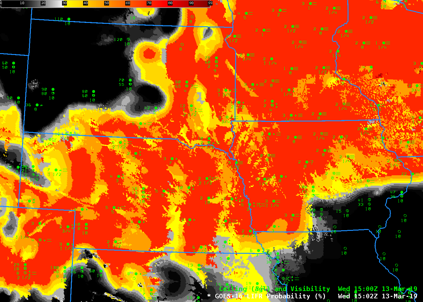
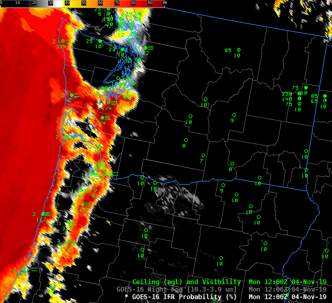
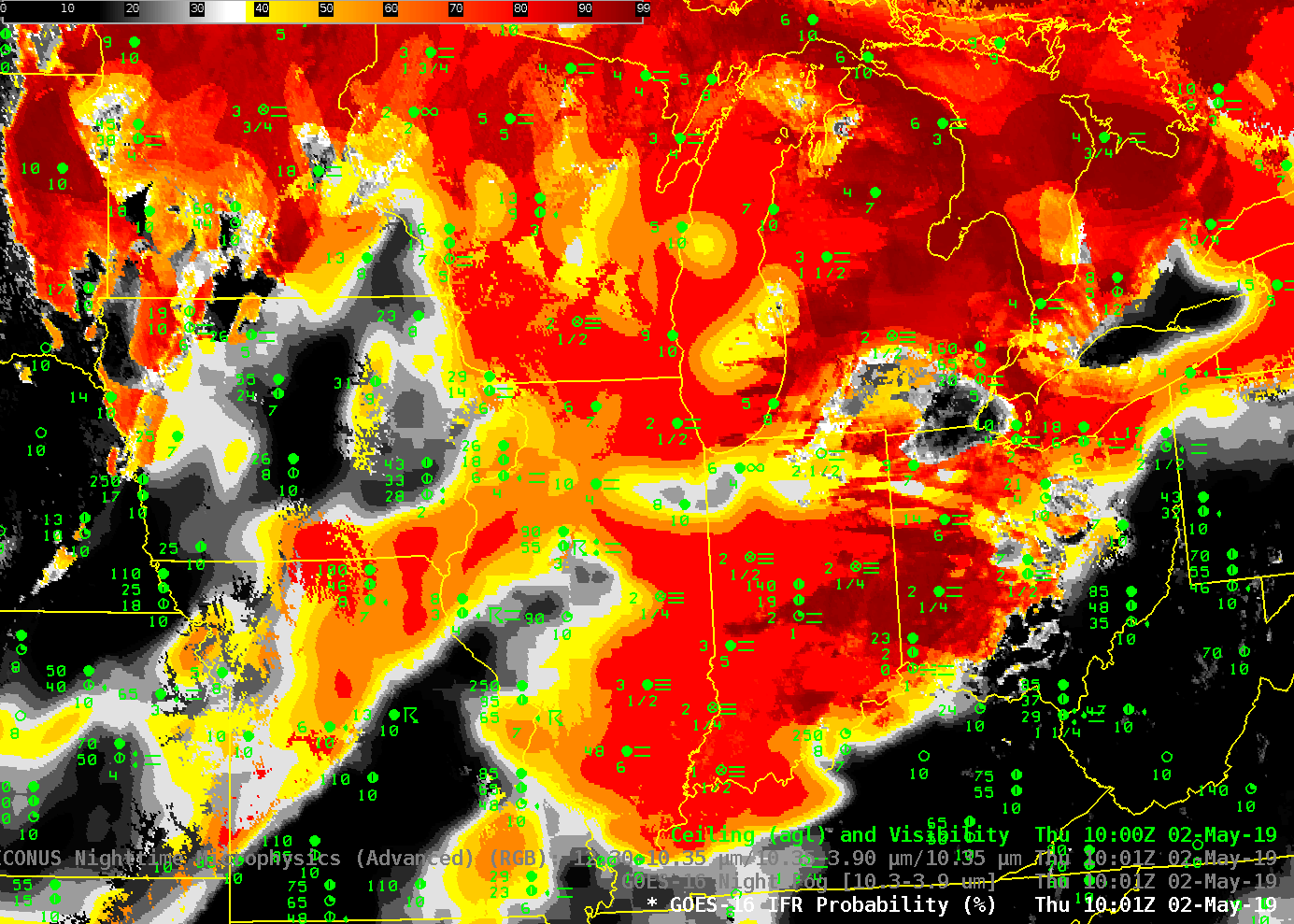
IFR Probability shows a a strong and consistent signal from Portland south to Eugene, and also over the Pacific, and north of Portland into the southern Puget Sound. In these regions, Rapid Refresh Model data are showing the presence of low-level saturation, a good indicator that IFR conditions may be present. IFR Probability shows small values under the region of low clouds detected by satellite over the Strait of Juan de Fuca; the Rapid Refresh model there is not showing low-level saturation. There is also a small signal in the clear skies over north-central Oregon where a brightness temperature difference is occurring because of soil-driven emissivity differences.

Use IFR Probability to ascertain the likelihood of fog underneath cirrus decks, or to determined the likelihood of stratus decks reaching the surface (that is, if stratus is actually fog).

Fog in the Mid-South on August 8th

GOES-R IFR Probability, 1002 UTC on 8 August 2019, along with surface reports of ceilings and visibility (Click to enlarge)

GOES-R IFR Probability fields from 1002 UTC on 8 August 2019, above, show a region of high probabilities mostly colocated with surface observations of ceilings and visibilities. IFR conditions are widespread from north of Memphis TN to southern Illinois. IFR Probability is a fused product, using both satellite imagery to detect low clouds and Rapid Refresh model data to identify regions of low-level saturation. Where both indicators are present (for example, over extreme western Kentucky and adjacent regions of southern Illinois and northwest Tennessee), IFR Probabilities are very high and IFR conditions are observed. There are also regions where only model data can be used — because satellites are not detecting low clouds (because high clouds are blocking the view); such a case is over northwest Arkansas, where IFR Probabilities are high (albeit not as high as over western Kentucky) and the field is not pixelated like a satellite image can be. IFR Conditions are observed there as well. (Click here for a screen shot from later in the morning of the Paducah National Weather Service office front page showing Dense Fog Advisories in Tennessee, issued by the Memphis Forecast Office).

The toggle below compares the IFR Probability field with the GOES-16 ‘Night Fog’ brightness temperature difference. There is no consistent signal in the brightness temperature difference field to indicate fog on the ground. The color enhancement for the brightness temperature difference is created so that teal to blue is positive. Clouds made of liquid water droplets — such as stratus, or fog — will have a strong positive value because of the emissivity properties of small water droplets. (That is, those droplets emit 10.3 µm radiation mostly as a blackbody would, but do not emit 3.9 µm radiation as a blackbody would). Note in particular the very dark enhancement over northwest Arkansas (suggestive of cirrus there that will block any satellite view of low clouds) and the grey enhancement over west central Tennessee, north of Memphis, where mid-level clouds are similarly blocking a good view of the stratus at the surface.

GOES-16 IFR Probability and GOES-16 ‘Night Fog’ Brightness Temperature Difference field (10.3 µm – 3.9 µm) at 1002 UTC on 8 August 2019 (Click to enlarge)

The Nighttime Microphysics RGB can also be used to alert forecasters to fog — but a main component of that detection is the Night Fog brightness temperature difference field, and where the Night Fog brightness temperature difference fails to identify fog, as above, Nighttime Microphysics will as well, as shown in the toggle below. Which color is useful for identifying fog in the RGB below? Almost all of them!

Fog and Low Stratus under cirrus

Night Fog Brightness Temperature Difference (10.3 µm – 3.9 µm), 0801-1311 UTC on 7 May 2019 (Click to animate)

Consider the animation above, of the Brightness Temperature Difference product (10.3 µm – 3.9 µm) centered on Colorado on the morning of Tuesday 7 May 2019. The surface observations show widespread IFR conditions, but because of widespread high clouds over the region, the brightness temperature difference shows little signal that is consistent with low clouds (blue or cyan in this enhancement). There isn’t much horizontal spatial correlation between observations of low ceilings/reduced visibility and the Brightness Temperature Difference product. When low clouds are overlain by high clouds, don’t expect a satellite detection of low clouds to work. Note also how the Brightness Temperature Difference field loses its signal as the sun rises and a general increase in the amount of reflected solar shortwave (3.9 µm) infrared radiation increases.

GOES-R IFR Probability includes near-surface information that is useful, especially when mid-level or high clouds obscure the satellite view of low clouds. Rapid Refresh estimates of near-surface saturation are used to gauge the probability of IFR conditions. In the case on 7 May 2019, that information allowed GOES-R IFR Probability to approximate exactly where the lowest ceilings and more reduced visibilities were. There is therefore a much better spatial correlation between the location of surface observations showing IFR conditions, and the IFR Probability field. This has a tacit implication on how well the Rapid Refresh Model is simulating the evolution of the atmosphere. Note also that in contrast to the Brightness Temperature Difference field, a consistent signal is maintained through sunrise.

GOES-R IFR Probability, and surface observations of ceilings/visibility, 0801-1311 UTC on 7 May 2019 (Click to animate)

Because the NightTime Microphysics RGB relies on the Night Fog Brightness Temperature difference field, it rises or falls on fog detection on the shoulders of the Brightness Temperature Difference field. On this day, it fell. Click here for the Nighttime Microphysics RGB animation; the animation below toggles between the three fields — Night Fog Brightness Temperature Difference, Nighttime Microphysics RGB, and IFR Probability — at 1002 UTC on 7 May 2019.

Night Fog Brightness Temperature Difference (10.3 µm – 3.9 µm), Nighttime Microphysics RGB and GOES-R IFR Probability fields, 1001 UTC on 7 May 2019 (Click to enlarge)

Fog surrounding convection in the Midwestern United States

GOES-16 IFR Probability and GOES-16 ‘Night Fog’ Brightness Temperature Difference (10.3 µm – 3.9 µm) at 1001 UTC on 2 May 2019, along with surface observations of ceilings and visibility (Click to enlarge)

Widespread Fog occurred over the midwestern United States on Thursday morning, 2 May 2019, with some Dense Fog Advisories issued. Some of the fog developed under an extensive cirrus canopy associated with strong convection over north-central Illinois, and those cloud layers make satellite-based detection of stratus near the surface (i.e., fog) a challenge. The toggle above between the Night Fog Brightness Temperature Difference (10.3 µm – 3.9 µm) and GOES-16 IFR Probability highlights the difficulty in using the brightness temperature difference alone to outline regions of fog. In contrast, the Rapid Refresh model information on low-level saturation allows IFR Probability to alert a forecaster to the likelihood of fog in regions underneath cirrus, regions such as southeastern Illinois and southwestern Indiana.

There is an excellent spatial correlation between regions with high IFR probability and low ceilings/reduced visibilities, and also with regions with low IFR probability and non-IFR conditions (central Iowa, for example, and central Illinois southwestward into central Missouri).

Because the Night Fog Brightness Temperature difference is a central feature of the Nighttime Microphysics RGB product — Night Fog Brightness Temperature difference is the green part of that RGB, as apparent in the toggle below — Nighttime Microphysics also is challenged to identify fog in regions under cirrus

Advection Fog and Multiple Cloud Layers

GOES-16 Night Fog Brightness Temperature Difference (10.3 µm – 3.9 µm), Low IFR Probability and Advanced Nighttime Microphysics RGB at 0837 UTC on 13 March 2019 (Click to enlarge)

An intense early Spring storm produced blizzard conditions over the western Great Plains on 13 March 2019 (See this blog post for example). The southerly flow in advance of the storm moved moist air over a dense snowpack over the upper Midwest, resulting in dense Advection Fog. The animation above cycles between the Night Fog Brightness Temperature Difference (10.3 µm – 3.9 µm), the Advanced Nighttime Microphysics RGB that uses the Night Fog Brightness Temperature Difference as the ‘green’ and GOES-16 Low IFR Probabilities.

At 0837 UTC, high clouds had not yet covered all of the upper Midwest, and the satellite still viewed stratus clouds over Wisconsin and Minnesota (bright cyan in the Night Fog Brightness Temperature difference enhancement). Note the difference in the Low IFR Probability field in regions where high clouds are present (Iowa and states to the south and west) and where they are not. Low IFR Probability has a pixelated look over Wisconsin because modest satellite pixel-level variability is included in the IFR probability field. Over Iowa, in contrast, satellite data gives no information about reductions to visibility under the thick cloud cover; low-level data from the Rapid Refresh model drives the Low IFR Probability field there. Probabilities are high in regions where observations suggest IFR/Low IFR conditions are present. This suggest the Rapid Refresh is simulating the evolution of the atmosphere well over the Plains.

The Advanced Nighttime Microphysics RGB can detect low clouds — but only when high clouds are not in the way. For this case, the RGB signal over Wisconsin is consistent with stratus and fog, but over Iowa the signal is consistent with cirrus that is occurring there. Surface restrictions in visibility and lowered ceilings are similar in the two states, and the IFR Probability field has similar values in the two states.

By 1502 UTC on 13 March (below), high clouds had overspread the entire Midwest; Low IFR Probability relies almost entirely on Rapid Refresh Model estimates of low-level saturation. That is why the field over northern Minnesota and northern Wisconsin is flat. Some holes in the high clouds are suggested by the pixelated look of the field in Iowa and southern Wisconsin.

GOES-16 Low IFR Probability, 1502 UTC on 13 March 2019 (Click to enlarge)

Fog under multiple cloud layers

GOES-16 Night Fog Brightness Temperature Difference (10.3 µm – 3.9 µm), 1137 – 1452 UTC on 31 October 2018 (Click to animate)

Consider the imagery above: The Night Fog Brightness Temperature Difference (10.3 µm – 3.9 µm) product can be used to highlight regions of low clouds (cloud made up of water droplets) because those water droplets do not emit 3.9 µm radiation as a blackbody (but do emit 10.3 µm radiation nearly as a blackbody), and the conversion of sensed radiance to brightness temperature assumes blackbody emissions. Thus, the 10.3 µm brightness temperature is warmer than at 3.9 µm. In the enhancement used, low stratus clouds are shades of cyan. Is there fog/low stratus along the coast of the Pacific Northwest? How far inland does it penetrate. It is impossible in this case (and many similar cases) to tell from satellite imagery alone because multiple cloud layers associated with a storm moving onshore prevent the satellite from seeing low clouds. The animation shows the Brightness Temperature Difference field along with surface reports of visibility and ceilings. IFR and near-IFR conditions are widespread, but there is little correlation between their location and the satellite-only signal.

GOES-16 Night Fog Brightness Temperature Difference (10.3 µm – 3.9 µm), 1137 – 1452 UTC on 31 October 2018, along with surface reports of ceilings (AGL) and visibility (Click to animate)

GOES-R IFR Probability fields fuse together satellite information and model data to provide a better estimate of where IFR conditions might be occurring. The animation below, for the same times as above, shows a high likelihood of IFR conditions (as observed) over much of the eastern third of Washington State. The satellite doesn’t give information about the near-surface conditions in this case, but the Rapid Refresh data strongly suggests low-level saturation, so IFR probabilities are high. The field also correctly shows small likelihood of IFR probailities over coastal southern Oregon and northern California. The Rapid Refresh data used have 13-km resolution, however; fog at scales smaller than that may be present — in small valleys for example.

GOES-16 IFR Probabilities, 1137 – 1452 UTC on 31 October 2018 (Click to animate)

IFR Probability can distinguish between stratus and fog

Night Fog Brightness Temperature Difference (10.3 µm – 3.9 µm). 1152 UTC on 11 October (Click to enlarge)

Consider the Night Fog Brightness Temperature Difference product, above. The enhancement is such that blue regions show where 10.3 µm brightness temperatures are warmer than brightness temperatures at 3.9 µm. At night, this occurs because cloud water droplets do not emit as much 3.9 µm radiation as a blackbody; the conversion of the sensed radiation to a brightness temperature assumes blackbody emissions have occurred, however, and as a result, the 3.9 µm brightness temperature is cool. Cloud water droplets do emit as a blackbody at 10.3 µm, so the brightness temperature over cloud water droplets is warmer than the it is at 3.9 µm. Blue, then, signifies stratus clouds in this enhancement. Can you tell where the fog is? Do you think IFR conditions are occurring wherever the Brightness Temperature Difference field is blue? How about under the extensive cirrus shield, associated with former Hurricane Michael, that is over the southeastern fifth of the image?

The Advanced NIght time Microphysics RGB for the same time, below, uses as one of its inputs (the ‘green channel’ in the RGB) the Night Fog Brightness Temperature Difference (Click here for a toggle between the two to reinforce that statement).

Night Time Microphysics RGB at 1152 UTC on 11 October (Click to enlarge)

GOES-R IFR Probability fields, below, for the same time are useful because Rapid Refresh model data used in IFR Probability include low-level model estimates of saturation. If saturation does not exist underneath the cloud deck, then IFR Probabilities are suppressed. Don’t expect fog, then, underneath the strong signal in the Brightness Temperature Difference field over most of the Midwestern United States! In addition, the Rapid Refresh Model data defines potential fog under the big cirrus shield over the Appalachians.

GOES-R IFR Probability fields at 1152 UTC on 11 October (Click to enlarge)

Click here for the Advanced Microphyics RGB with observations of ceilings and visibility. Here are the observations over the Brightness Temperature Difference. Observations plotted on top of IFR Probability are shown below.

GOES-R IFR Probability fields at 1152 UTC on 11 October along with surface observations of ceilings and visibilities (Click to enlarge)

GOES-R Fog Product Examples

Fog detection fusing GOES, Terra/Aqua or Suomi/NPP Satellite data with Model output