Monthly Archives: August 2012

Excellent example of the importance of model data

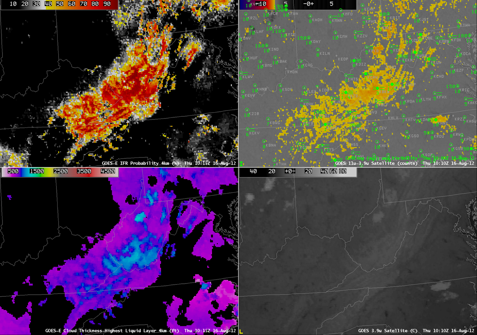
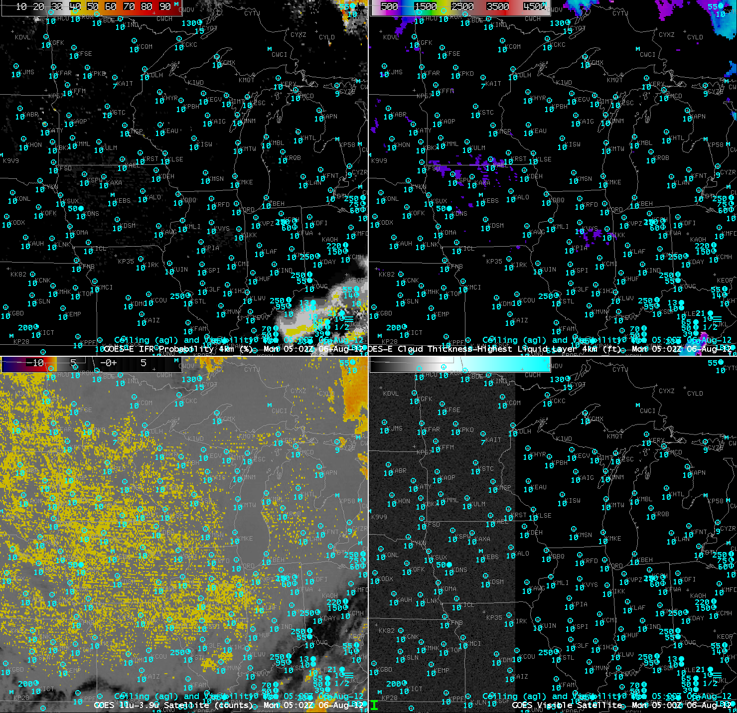
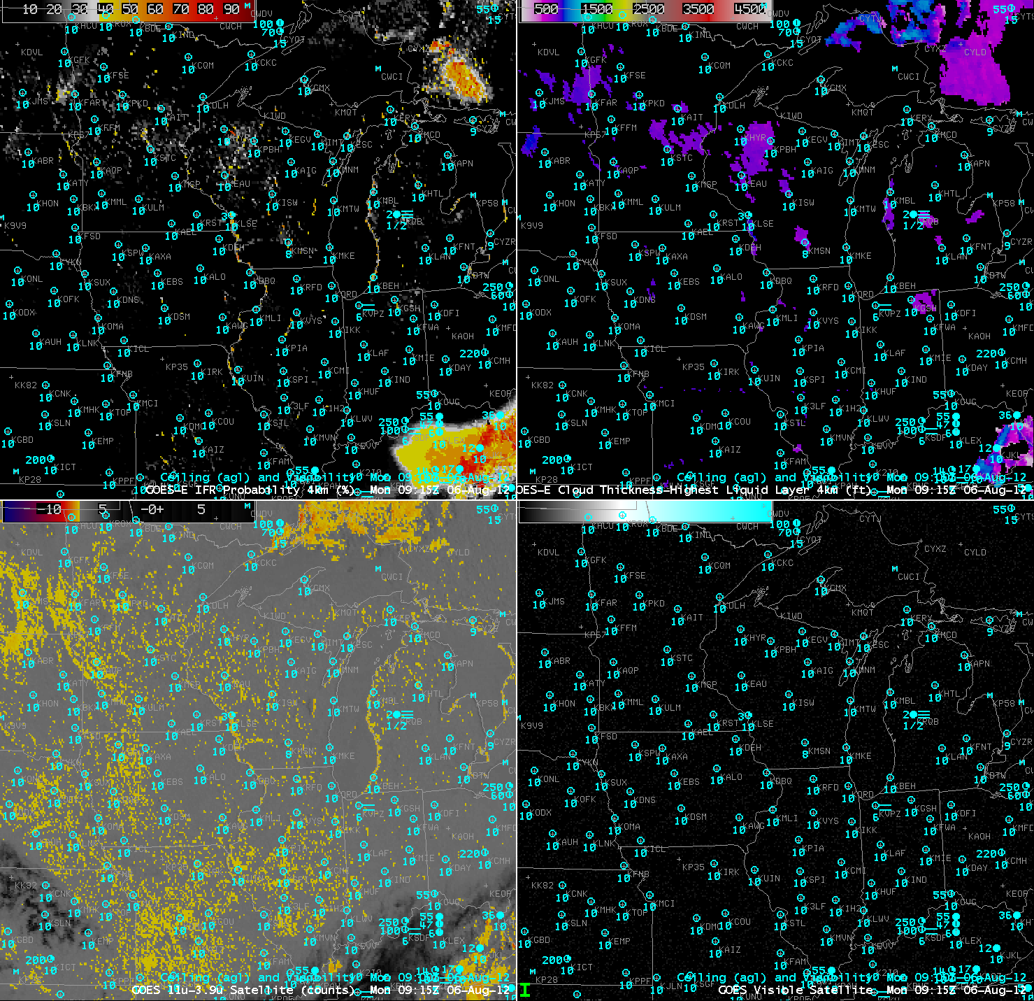
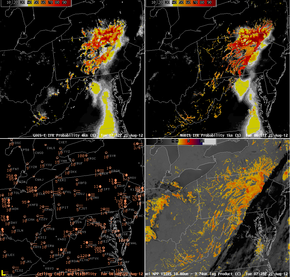
GOES-R IFR Probabilities computed using GOES-East data (Upper Left), GOES-R IFR Probabilities computed using MODIS data (Upper Right), Surface Observations and Cloud Ceilings Above Ground level (Lower Left), Suomi-NPP VIIRS Brightness Temperature Difference field, 10.8  µm – 3.74 µm (Lower Right).  Times as indicated.

Three different satellite sensors — the GOES Imager on GOES-East, MODIS on Aqua, and VIIRS on Suomi/NPP — viewed data from the occurrence of Valley Fog over the Appalachians (and surroundings) early in the morning of 21 August.  A shortcoming of the Brightness Temperature Difference field in the lower left is immediately apparent:  no fog/low stratus is indicated where high clouds exist, even though observations do show IFR conditions.  In contrast, the fused product does show heightened probabilities underneath that high cloud deck.  Probabilities are not as high as they are where both satellite and model predictors can be used to evaluate the presence of fog and low stratus, and the resolution of the field is different, obviously limited to the horizontal resolution of the Rapid Refresh, meaning that small river valleys, that are very obvious in the regions where satellite data are used (and even much more obvious when high-resolution MODIS or VIIRS data are used).  Note also how GOES-R IFR Probabilities de-emphasize the signal over western Ohio, where IFR conditions are not reported.  Brightness temperature difference fields from MODIS and from GOES both see a signal there, as also shown in the VIIRS field, but these stratus clouds are not obstructing visibility.

Bottom line:  MODIS data’s higher resolution observes the big differences between river valleys and adjacent cloud-free ridge tops.  GOES-East has difficulty in resolving those differences.  So MODIS IFR fields better highlight river fog.  Model data can help discern between fog on the ground, and stratus that is off the ground.

Cloud thickness as a predictor of Fog Dissipation

GOES-R IFR Probabilities (Upper Left), GOES-R Cloud Thickness (Upper Right), GOES-East 10.7 µm imagery (Lower Left) and GOES-East 0.63 µm (Visible) imagery (Lower Right)m at 1045 and 1402 UTC

Radiation fog occurred over central Lower Michigan near Saginaw overnight into the morning of the 20th of August, and the thickest fog is indicated at 1045 UTC — just before sunrise — to be just shy of 1000 feet thick.  This fog bank slowly shifted southward, and dissipated shortly after 1400 UTC, one county south of its location at 1045 UTC.  That dissipation time neatly fits in with the graph of fog thickness vs. dissipation time shown here.

Interpreting the GOES-R IFR Product in regions where Model and Satellite Predictors are used

GOES-R IFR Probabilities computed from GOES-East and from the Rapid Refresh, hourly from 2202 UTC on 19 August through 1402 UTC on 20 August

The animation above demonstrates the different ways in which GOES-R probabilities can be detected, and the values that can occur.  Much of the East Coast was under a multi-layer cloud deck (as shown below in the color-enhanced 0632 GOES-East 10.7 µm image).  In those places, IFR probabilities will be computed using Rapid Refresh model output, and the character of the IFR probability field will differ from how the field looks when satellite data are used as IFR predictors.

For example, the smooth IFR probability field over North Carolina in this loop (especially from 0300 UTC to 0700 UTC) strongly indicates model-only predictors.  Before and after that time there are small regions that are more pixelated, suggesting satellite input.  At 0600 UTC, GOES-R IFR probabilities start to increase over West Virginia as overnight cooling allows temperatures to approach the dewpoint, and fog starts to develop.  Probabilities become quite high by sunrise over and near West Virginia, and IFR conditions are evident.  IFR probabilities where satellite and model data are used as predictors — as over West Virginia — are generally higher than regions where model data only are used (over North Carolina).  Model data will always be included in the computation of IFR probabilities.  In regions of multiple cloud layers, such as over North Carolina, it is used alone and IFR probabilities can be high.  In regions of low clouds, such as over West Virginia, the model underscores what the satellite data are telling and IFR probabilities will be even higher.  There can also be regions where the Satellite and Model predictors give conflicting information on the presence of fog/low stratus.  In these regions, IFR probabilities will be somewhat lower.

Note that the terminator is present in this loop, both at sunset (2345 UTC) and at sunrise (the 1100 UTC imagery).  The change in IFR probabilities that occur is evident as predictors that are used during the day change to or from those used at night.  At 1100 UTC, probabilities are increasing by about 18% over North Carolina.

GOES-13 10.7 µm imagery at 0632 UTC on 20 August 2012.

Fog and Low Clouds after evening Convection

GOES-R IFR Probabilities (Upper Left), Brightness Temperature Difference (10.7 µm – 3.9 µm) (Upper Right), GOES-R Cloud Thickness (Lower Left), GOES-East 3.9 µm Brightness Temperature (Lower Right), for 0315 UTC to 1115 UTC on 17 August 2012

Post-sunset convection can supply the moisture that is needed for the development of overnight fog and low stratus.  But do those low clouds cause IFR conditions?  This example over NW Arkansas from the morning of 17 August shows GOES-R IFR Probabilities that successfully pinpoint the regions where IFR conditions are most likely and exclude regions where IFR conditions do not occur.  The brightness temperature difference field and the 3.9 µm both show convection before 0600 UTC. Subsequent to the convection, a brightness temperature difference signal that is consistent with fog/low stratus does develop over southern Kansas, and then over south-central Missouri and northwest Arkansas.  The GOES-R IFR Probabilities, however, suggest that IFR conditions are likely only over northwest Arkansas (where IFR conditions are observed).

This example also ably demonstrates the differences in the character of the IFR Probability field that occur when model data alone are used to predict IFR probabilities (Northeast Arkansas during most of the loop) vs. a combination of Satellite and Model data (Northwest Arkansas at the end of the loop).

Valley Fog over Appalachia

GOES-R IFR Probabilities (Upper Left), Brightness Temperature Difference (10.7 micrometers – 3.9 micrometers) (Upper Right), GOES-R Cloud Thickness (Lower Left), GOES-East 3.9 micrometer imagery (Lower Right)

The radiation fog example over West Virginia and surrounding states on 16 August highlights characteristic strengths of the GOES-R Fog/Low Stratus products.  Note, for example, how the enhanced brightness temperature field shows no apparent signal over the Ohio River Valley along the western border of West Virginia, despite the presence of IFR conditions at Pt. Pleasant (K3I2) and Huntington (KHTS).  In contrast, the IFR probability does the suggest the possibility of visibility obstructions in the valley.

Note the region of low cloud over north-central North Carolina.  The feature is quite apparent in the 3.9-micrometer imagery, and the brightness temperature difference field also has a maximum return there.  This cloud is likely elevated stratus (brightness temperatures were generally in the single digits Celsius), and the IFR Probability field correctly diminishes the strong satellite predictor signal there.

Satellite and Model Predictors of Fog

GOES-R IFR Probabilities (Upper left), Enhanced GOES-East 10.7 micrometer imagery (Upper right), Rapid Refresh Mean Relative Humidity (1000-850 mb) (Lower left), Composite Radar Reflectivity (Lower right).  Times as indicated.

A large convective system moved over Wisconsin during the morning of 16 August 2012 and it illustrates the importance of fused data in diagnosing IFR conditions.  The deep convective cloud precludes any satellite detection of low water-based clouds, so the traditional method of detecting fog/low stratus (the brightness temperature difference between 10.7 and 3.9 micrometers) cannot be used.  In this case, model data, in the form of Rapid Refresh Relative Humidity, is used to fill in regions where satellite predictors cannot help.  Note the observation of IFR conditions at Wisconsin Rapids (KISW);  this is a region of very high model relative humidity.  Model relative humidity is just as high over south-central Minnesota;  in that region, however, satellite predictors do exist, and they do not suggest fog/low clouds, so the IFR probability there is comparitively lower.

The character of the IFR probability field is much less pixelated in regions where model data only are used as predictors.  When satellite data and model data are used, as over northwest Wisconsin, for example, the pixelated nature of the satellite data becomes apparent.

Radiation Fog over Kansas

GOES-R IFR Probabilities (Upper left), GOES-East brightness temperature difference (Upper Right), GOES-R Cloud Depth (of lowest liquid layer) (Lower Left), GOES-East Visible Imagery (Lower Right) from 0345 UTC through 1645 UTC on 15 August 2012.

Radiation fog that developed over Kansas early in the morning of August 15th highlights the strengths of the GOES-R IFR algorithm.  IFR probabilities are highest in regions where the satellite signal — the brightness temperature difference — is strong;  IFR probabilities are reduced in regions where the model signal is not strong.  Thus, IFR probabilities are generally highest in regions where IFR conditions are observed.  In the loop above, high IFR probabilities do not extend into central Kansas where a satellite signal does exist.  In addition, the GOES-R IFR imagery at 0502 UTC does not include the sudden expansion in areal coverage (likely due to stray light) that appears only at that time.  The IFR Probability signal persists through sunrise (in contrast to the Brightness Temperature Difference signal that flips sign as the sun comes up).  GOES-R Cloud thickness peaks around 1200 feet at the last image before twilight;  according to this chart, that suggests that the radiation fog will burn off more than 4 hours after sunrise.  The last fog did not dissipate until shortly after 1600 UTC.

The Challenge of Identifying Fog in River Valleys

Animation of GOES-R IFR probabilities computed from GOES-East (upper left), Brightness Temperature difference (11 – 3.9) from GOES-East (upper right), Surface visibilities and ceilings and GOES-East Visible imagery (lower left), GOES-R IFR probabilities computed from MODIS (lower right)

Radiation fog that forms first — or only — in river valleys is a challenge to detect.  In the example above from Pennsylvania for the morning of August 8 2012, the satellite signal starts to appear over the West Branch of the Susquehanna around 0500 UTC.  It is very unlikely that a numerical model with a horizontal resolution of (only) 13 km — such as the Rapid Refresh — will be able to forecast the development of such a small-scale feature, so the satellite observations are key.  Nominal 4-km resolution of the infrared channels is the principle limiting factor in detection.

The presence of high clouds over southeast Pennsylvania precludes the detection by satellite of low clouds/fog, so the GOES-R IFR product there is driven primarily by model output, and the scale of the river fogs are simply too small to be simulated in the model.  Fog probabilities do increase near Selinsgrove (KSEG) around daybreak because the model relative humidity does reach high enough values.  This also happens over southeast Pennsylvania.  Typically, model relative humidities in the lowest kilometer of the model must be greater than 80-85% for a strong GOES-R IFR signal to be present.

GOES-R IFR probabilities computed from GOES-East (upper left), Brightness Temperature difference (11 – 3.9) from GOES-East (upper right), Surface visibilities and ceilings and GOES-East Visible imagery (lower left), GOES-R IFR probabilities computed from MODIS (lower right), all valid at 0700-0715 UTC 8 August 2012

Note that at 0715 UTC there is a comparison between the better resolution of the MODIS imagery.  When GOES-R is operational, resolution will be in between that of current GOES and MODIS.  The MODIS GOES-R IFR probabilities are much higher, and show the different river valleys far more cleanly than present GOES.

IFR Probabilities under clouds

GOES-R IFR Probabilities (from GOES-East) (upper left), GOES-East Brightness Temperature Difference 11 µm – 3.9 µm (upper right), Plot of Ceiling (AGL) and visibility (lower left), Enhanced 11 µm brightness temperature (lower right) from 0815 UTC from 1845 UTC on 7 August 2012

When atmospheric conditions support multiple cloud layers and low-level fog, the heritage method of fog/low cloud detection (the brightness temperature difference between the 10.8 and 3.9 µm channels) will yield little information because the highest cloud will likely include ice, and the brightness temperature difference exploits emissivity differences in water clouds.  In these regions, the model output is vital to predict IFR probabilities.  Because satellite predictors are giving no information in these regions, however, the overall probabilities are likely to be lower than the case where both satellite and model suggest the presence of fog.  Expect the highest probabilities when both satellite model suggest the presence of fog.  If only one of the predictors (satellite data or model data) suggests the presence of fog, IFR probabitilies will be lower.

In the example above, periodic episodes of IFR conditions are occurring over Georgia.  Most of the IFR probability signal is coming from the Rapid Refresh, and there are hints that the model output is not quite reproducing the observed weather.  If satellite data are not used as a predictor in the GOES-R IFR Probability product (because of high clouds), interpretation of the GOES-R IFR product is complicated by Rapid Refresh performance.

Resolution and River Valleys

Animation of GOES-R IFR probabilities (upper left), GOES-R Cloud Thickness (upper right), GOES-East Brightness Temperature Differences (lower left), and Visible Imagery (lower right), from 0400 through 1400 UTC on 6 August 2012

River Valleys — sources of moisture — are nearly sub-pixel scale in GOES-East imagery.  Thus, any signal that develops in a river valley will likely take time to appear, and an example of that occurred over the upper Midwest on the morning of August 6th.  The signal develops along the river starting around 0800 — 0900 UTC (LaCrosse, WI, starts to report visibility and ceiling obstructions at 1000 UTC).  There are several interesting aspects in the loop.

GOES-R IFR probabilities (upper left), GOES-R Cloud Thickness (upper right), GOES-East Brightness Temperature Differences (lower left), and Visible Imagery (lower right), at 0502 UTC on 6 August 2012

The imagery at 0502 UTC (above) shows the result of stray light contamination on the brightness temperature difference field (lower left), but this increase in signal over the Plains is ephemeral, and it is gone in 15 minutes.  There is also an increase in the brightness temperature difference signal over the Plains as sunrise approaches.

GOES-R IFR probabilities (upper left), GOES-R Cloud Thickness (upper right), GOES-East Brightness Temperature Differences (lower left), and Visible Imagery (lower right), at 0915 UTC on 6 August 2012

By 0915 UTC, the GOES-R IFR probabilities have increased slightly along the Wisconsin River in southwest Wisconsin, as has the brightness temperature difference signal (although that signal has increased elsewhere as well where the GOES-R IFR probabilities remain low).  Compare the (relatively) low-resolution GOES-based imagery to the higher resolution Suomi/NPP resolution discussed here.  Note also how the GOES-R IFR probability product correctly suppresses the IFR probabilities over Iowa and Missouri where observations show no obstructions to visibility.