Monthly Archives: July 2013

Fog Detection under Cirrus

MODIS Brightness Temperature Difference and MODIS-based GOES-R IFR Probabilities, 30 July 2013, 0835 UTC

MODIS Brightness Temperature Difference and MODIS-based GOES-R IFR Probabilities, 30 July 2013, 0835 UTC

The toggle above switches between a brightness temperature difference field and a GOES-R IFR Probability field (both from MODIS) over Missouri and Kansas (including the busy airport in Kansas City).  The cirrus shield over the convective complex over Missouri obscures any satellite view of low clouds.  North and west of that cirrus shield, over Nebraska, Kansas and Iowa, the brightness temperature difference indicates clouds comprised of water droplets (that is, stratus or fog).  Ceilings and visibilities underneath the cirrus canopy, and within the stratus deck show regions of IFR conditions. Rapid Refresh model data that is part of the GOES-R IFR Probability algorithm is able to alert a viewer (or forecaster) to the possibility of Fog/Low stratus in areas underneath the cirrus. Probabilities under the cirrus canopy are lower because satellite-based predictors are not used in the computation of probabilities.


Unusual late-July High Plains Fog

GOES_IFR_PROB_20130729_loop

Fog and low stratus developed over the High Plains under easterly (upslope) flow in the early morning hours of July 29, 2013, and the GOES-R IFR Probability fields ably discriminated between regions of stratus and visibility-restricting low stratus/fog.  Note in the imagery above how the Brightness Temperature Difference field (upper right) includes a strong signal over eastern Nebraska where visibility restrictions/low ceilings are not present.  Fusing the satellite data with Rapid Refresh model data allows the MODIS and GOES-based GOES-R IFR Probability fields to more accurately depict the regions of low visibilities/ceilings.  Note that the brightness temperature difference product from MODIS, below (Lower Right), also highlights the mid-level stratus over eastern Nebraska.

MODIS_FOG_20130729_0521

Low clouds in the Pacific Northwest

GOES-R IFR Probabilities computed from GOES-West (Upper Left), GOES-West Brightness Temperature Difference (10.7 µm – 3.9 µm) (Upper Right), GOES-R Cloud Thickness from GOES-West (Lower Left), GOES-R IFR Probabilities computed from MODIS (Lower Right), hourly from 0500 through 1200 UTC on 23 July 2013.

Hourly GOES-R IFR Probabilities ably capture the creep of low fog and stratus into Puget sound from the north — through the strait of Juan de Fuca, and from the south, with low clouds eventually surrounding the Olympic Mountains.  Part of the input into the GOES-R IFR Probability algorithm is the brighness temperature difference shown in the upper right, and note that it used alone overpredicts where low clouds/fog might be occurring.  Including Rapid Refresh data allows the GOES-R algorithm to restrict — correctly — the IFR conditions to where they are most widespread.

Suomi-NPP data from the VIIRS instrument includes a Day/Night band that on July 23rd, when the moon was approaching full, neatly outlines both the cloudy regions — where moonlight is reflected off clouds — and those regions where light is being emitted (that is, cities).

As above, but with the VIIRS Day/Night band in the bottom right, at 0923 and 1103 UTC.

Suomi/NPP VIIRS data also includes 10.8 and 3.74 µm imagery, so a brightness temperature difference product can be computed (work is in progress to incorporate Suomi/NPP data into the GOES-R algorithm suite so an NPP-based IFR probability can be developed.  The toggle below compares the day/night band data with the brightness temperature difference produce at 0923 UTC.

Cloud thickness as a Predictor for dissipation time

GOES-R IFR Probabilities (Upper Left) computed from GOES-East data, Brightness temperature difference (GOES-East, 10.7 – 3.9 ), GOES-R Cloud Thickness (Lower Left), Suomi-NPP Day/Night Band (Lower Right).  All images hourly, 0515 UTC through 1115 UTC on 22 July 2013.

When fog forms overnight because of radiational cooling to the dewpoint, the thickness of the fog is related to the time it will take for the fog to dissipate.  In general, thick fog dissipates more slowly than thin, and because thick fog is generally surrounded by thinner fog, a region of fog/low stratus will generally erode from the outside in.  The animation above shows the gradual development and expansion of fog overnight over Iowa, Illinois and Missouri, with thicknesses over southeastern Iowa eventually reaching values of 1100 feet!

The relationship between time of dissipation and fog depth is shown on this chart, where the depth is the last pre-twilight image.  For 22 July 2013, that image is at 1045 UTC, shown below.  A value of 1100 feet corresponds to a dissipation time of 2-3 hours after sunrise.

As above, but for 1045 UTC 22 July 2013

The visible animation, below, shows dissipation between 1400 and 1500 UTC.

GOES-13 Visible imagery, 1215 through 1545 UTC 22 July 2013

Suomi/NPP data showed a snapshot of the fog development in this region at ~0800 UTC.

As above, but with a toggle of the Day/Night band and a Brightness Temperature Difference, all imagery at 0802 UTC 22 July 2013.

Fog development over the lower Mississippi River valley as viewed by different satellites

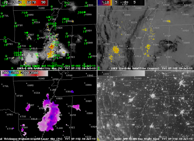
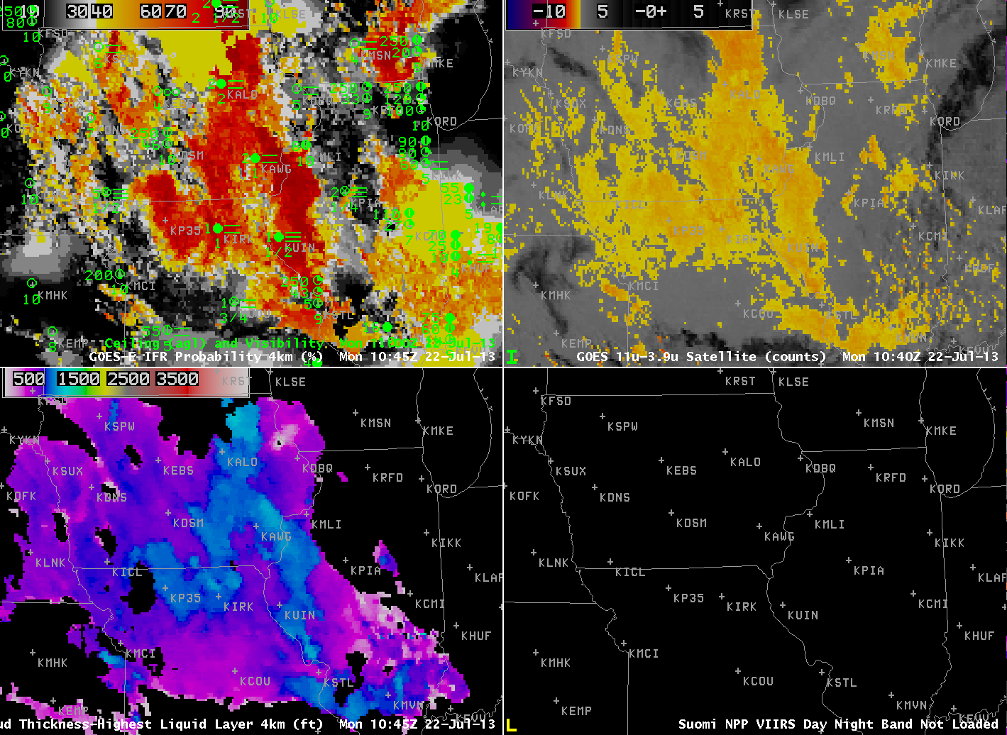
GOES-R IFR Probabilities computed from GOES-East (Upper Left), GOES-East Brightness Temperature Difference (10.7 µm – 3.9 µm) (Upper Right), GOES-R Cloud Thickness (Lower Left), GOES-East Visible Imagery (Lower Right), all images hourly from 0415 UTC through 1415 UTC 19 July 2013

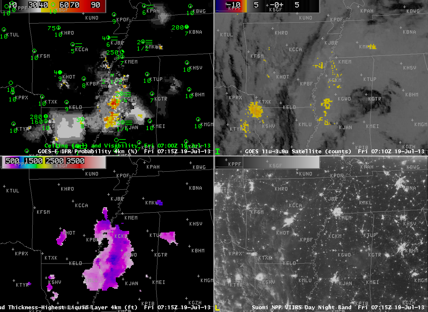
Hourly imagery of GOES-R IFR Probabilities show the development of high probabilities in a region where low clouds and fog develop to cause IFR and near-IFR conditions in and around the lower Mississippi River Valley.  The traditional method of detecting low stratus will be hampered by an abundance of high and mid-level clouds (as evidenced in the brightness temperature difference product, above, and in the day/night band imagery, below).  Different polar-orbiting satellites can give snapshots at high spatial resolution that describe the fog/low cloud fields.  The Suomi/NPP overpass at  0715 UTC (early in the night for radiation fog development), shows the abundance of high clouds over the western part of the domain, for example, that are illuminated by the setting half-moon.  It is difficult to discern low clouds in regions where IFR probabilities are high.

As above, but with Suomi/NPP Day/Night Band (Bottom Right), 0715 UTC.

 MODIS data are used to produce IFR probabilities, and those images are shown below.  The later of the images matches the time of the Suomi/NPP band shown above.

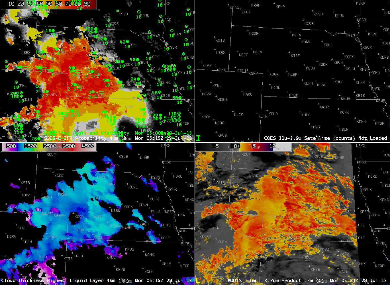
As above, but with MODIS-based GOES-R IFR Probabilities (Lower Right), at 0445 and 0715 UTC 19 July 2013

MODIS-based IFR probabilities are higher than GOES-based probabilities over the west-central part of Mississippi where satellite data are included in the predictors.  This occurs when the MODIS-based satellite signal of low clouds is stronger than that from GOES, which difference in signal can occur because of the finer resolution of the MODIS data.  In central Arkansas and northern Louisiana, however, where high clouds are present (and therefore where Satellite data are not used in the computation of the IFR Probability), the GOES-based and MODIS-based fields are nearly identical.

AVHRR data (below) can also be used to compute brightness temperature differences, but those data are not yet incorporated into the GOES-R algorithms.  However, the trend of the brightness temperature difference field can be used to monitor trends in low clouds/fog.  High clouds will obscure the view, however.  It is very difficult to infer a change in the amount of fog, and the concomitant decreases in visibility, based on the brightness temperature difference changes displayed below.

As above, but with the AVHRR Brightness Temperature Difference (10.8 – 3.74), bottom right, at 0654 UTC, 0837 UTC and 1051 UTC on 19 July 2013.

IFR Conditions over southwest mainland Alaska

Hourly GOES-R IFR Probability fields over southwest Alaska, 0500 to 1700 UTC 15 July 2013

The IFR Probability fields over southwest Alaska early on July 15 2013 show the influence of multiple cloud layers moving northward out of Bristol Bay and the Bering Sea starting near 0900 UTC.  IFR probabilities drop (because satellite data are not included as predictors when multiple cloud layers exist), and the field becomes flatter.  That is, it has less horizontal variability (especially compared to its pixelated nature when satellite data are included).  IFR conditions are largely confined to within the region of high IFR probabilities.

Two obvious boundaries are present in the field.  At 0800 UTC, a boundary extends southwest to northeast, with higher values to the north and west.  At 1500 UTC, a boundary extends southeast to northwest with higher values to the north and east.  In both cases, this line is the terminator, and daylight is occurring north of the line.  In general, IFR probabilities increase during the day (where they are diagnosed) because the cloud-clearing algorithm operates with a lot more certainty when visible imagery can be used to identify clouds.

MODIS data can be used in Alaska because Alaska’s high latitude ensures that MODIS overpasses are frequent (especially along the north slope of Alaska).  Three overpasses could be used between 0700 and 1415 UTC over this small region of southwest Alaska to give high-resolution depictions of IFR probabilities.  Using these high-resolution images with the high temporal resolution available from GOES-West gives a full description of the IFR Probability field over Alaska.  The 0832 UTC image suggests multiple cloud layers are still over Bristol Bay/the Bering Sea, and the 1415 UTC image shows both the day-night boundary and an IFR Probability field determined largely by model data.

MODIS-based GOES-R IFR Probabilities over southwest Alaska, 0654 UTC, 0832 UTC and 1415 UTC 15 July 2013

IFR Conditions over Georgia on a Summer Morning

Animation of GOES-East Water Vapor Imagery (6.7 µm), Brightness Temperature Difference Product (10.7 µm – 3.9 µm) and GOES-R IFR Probability computed with GOES-East data, 1000 UTC on 11 July 2013

The satellite animation, above, shows ample evidence of multi-layered clouds over Georgia and surrounding states, in a region where ceilings and visibilities approached/exceeded IFR conditions.  The traditional method of determining regions of fog/low stratus — the brightness temperature difference between the 10.7 µm and 3.9 µm channels — gives no information here because low clouds are screened by higher ice-phase clouds.

GOES-R IFR Probability fields merge information from GOES Imager data and the Rapid Refresh Model.  Even if GOES Imager data gives little information, GOES-R IFR Probability fields will give valuable information because they are also use information from the Rapid Refresh model.  Because the IFR Probability fields don’t include satellite data, probabilities are lower.  The large region of yellow — IFR Probabilities around 40% — sits over many stations that are reporting IFR conditions.   Note how IFR Probabilities are higher over North Carolina where satellite data are being used in the computation of the field — but there are fewer reports there of IFR conditions (despite the higher probability).  Temper the interpretation of the IFR Probabilities with knowledge of what is being used to compute them.

The evolution of IFR Probability fields can give a Head’s Up to deteriorating conditions in the atmosphere.  Note in the hourly animation below how probabilities initially do increase over regions that subsequently have IFR or near-IFR conditions.  At the end of the animation, there is an obvious boundary between different probabilities over northeast Georgia (Orange values around 55%) and western Georgia (values around 40%).  That southeast-to-northwest boundary shows where nighttime predictors are being used (to the west) vs. daytime predictors (to the east) in the computation of IFR Probabilities.

GOES-R IFR Probabilities (hourly) from 0200 through 1100 UTC, 11 July 2013

Resolution and Cloud Depth

GOES-R Cloud Thickness computed from GOES-East and from MODIS data, ~0815 UTC 9 July 2013

The resolution and view angle of MODIS, compared to the GOES Imager, means that smaller features are better resolved and more accurately navigated.  In the example above, the Kickapoo River in Vernon, Richland and Crawford Counties in southwest Wisconsin is clearly delineated in the MODIS product, with a small ribbon of values from 800-1000 feet, but not in the GOES where values are closer to 600.  Differences along the coast of Lake Michigan are also evident.  MODIS detects a thick cloud bank off the coast of Sheboygan County (the cloud thickness is near 1000 feet);  GOES detection has thicknesses of 800 feet in that region, but the values are shifted onshore because of parallax and the co-registration error that exists between the 10.7 µm and 3.9 µm  channels on the GOES-13 Imager.

If you are using Cloud Thickness to estimate fog dissipation, the difference between 1000 and 800 feet equates to 60-90 minutes.

Lake Superior Plus High Dewpoints Means Fog

GOES-R IFR Probabilities computed from GOES-East, and surface observations of ceilings/visibilities (Upper Left), GOES-East Brightness Temperature Difference (10.7 µm – 3.9 µm) (Upper Right), GOES-R Cloud Thickness computed from GOES-East (Lower Left), GOES-R IFR Probabilities computed from MODIS (Lower Right)

The combination of cold Lake surface temperatures in the 40s and 50s over Lake Superior and mid-Summer dewpoints in the 60s to near 70 is a recipe for fog over the upper midwest. North winds behind a complex of thunderstorms fostered the development of fog and low stratus over the upper midwest early in the morning on July 8th, as shown in the imagery above.

The GOES-R IFR Probability fields seamlessly track the expansion of fog/low stratus in the region around western Lake Superior;  highest probabilities are confined to regions where IFR or near-IFR conditions are observed.  The IFR Probabilities also downplay regions where the brightness temperature difference field is showing a signal (northwest Minnesota) but where visibility obscurations are small.

IFR Probabilities are not as large over southern upper Michigan or over north-central Wisconsin, regions where multiple cloud layers mean that the satellite component does not contribute to IFR Probability computation, resulting in a smaller value.  Note that Cloud Thickness is not initially computed there either:  Cloud Thickness describes the thickness of the lowest water-based cloud layer in non-twilight conditions.  If there are multiple cloud layers that include mixed-phase of ice clouds, cloud thickness is not computed.  Note also that cloud thickness is not computed in the hours around sunrise (i.e., during twilight conditions).

By 1702 UTC, the final image, the Summer Sun has burned off much of the fog and low stratus, with the exception being along the shorline of Lake Superior.  MODIS-based IFR Probabilities have much sharper edges because of the higher resolution of the MODIS instrument compared to the GOES Imager.

Fog Development over central Illinois

GOES-R IFR Probabilities computed from GOES-East, hourly from 0215 UTC through 1115 UTC on July 5 2013

GOES-R IFR Probabilities show a characteristic increase over central Illinois as radiation fog develops in the early morning hours of July 5 2013.  Probabilities are initially low, but gradually increase, and spread, as the fog develops.  The IFR probability field over Tennessee, Indiana and Kentucky has the characteristic flat look of a field produced mainly from model fields:  the probability field is flat, and IFR probabilities are low.  There are regions — such as near Nashville at the end of the animation — where the field includes satellite data;  IFR Probabilities there are larger and the IFR Probability field has a more pixelated appearance.

If multiple cloud layers are present, you should not expect the GOES-R Cloud Thickness product to yield a value.  GOES-R Cloud Thickness diagnoses the thickness of the highest water-based cloud in non-twilight conditions.  If ice clouds (or mixed phase) clouds are present, cloud thickness will not be computed.  The toggle below shows cloud thickness, GOES-R IFR Probabilities, and the Brightness Temperature Difference (10.7 µm – 3.9 µm)

GOES-R IFR Probabilities, GOES-R Cloud Thickness, and GOES-East Brightness Temperature Difference, 0730 UTC on 5 July 2013

There a several things of note in the image above.  IFR Probability field in central Illinois have higher values south of the peak in the brightness temperature difference field, where the lowest visibilities and ceilings are reported.  GOES-R Cloud Thickness is unavailable in regions underneath the high clouds in the eastern part of the imagery — over Tennessee and Kentucky, except where there are holes in the clouds.  Note how these regions of diagnosed GOES-R Cloud Thickness overlap with regions of pixelated GOES-R IFR Probability fields.  In both fields, Satellite data are being used for the computation.