Category Archives: Cloud Thickness

GOES-R IFR Probability gives information in the day too!

GOES-R IFR Probability from GOES-East (Upper left), GOES-East Visible (Upper Right), GOES-R Cloud Thickness (Lower left) and GOES-East Brightness Temperature Difference (Lower Right)

The GOES-R IFR Probability serves a useful purpose in the day:  It highlights where, in a field of clouds, the lowest visibilities and ceilings are likely.  In the image above from coastal North and South Carolina and Georgia. cloudiness is hugging the coast, as indicated both in the visible and in the tradiational brightness temperature difference product.  Highest probabilities of IFR conditions are depicted near Statesboro and Savannah GA, where ceilings and visibilities are lowest.

Cloud thickness as a predictor of Fog Dissipation

GOES-R IFR Probabilities (Upper Left), GOES-R Cloud Thickness (Upper Right), GOES-East 10.7 µm imagery (Lower Left) and GOES-East 0.63 µm (Visible) imagery (Lower Right)m at 1045 and 1402 UTC

Radiation fog occurred over central Lower Michigan near Saginaw overnight into the morning of the 20th of August, and the thickest fog is indicated at 1045 UTC — just before sunrise — to be just shy of 1000 feet thick.  This fog bank slowly shifted southward, and dissipated shortly after 1400 UTC, one county south of its location at 1045 UTC.  That dissipation time neatly fits in with the graph of fog thickness vs. dissipation time shown here.

Fog and Low Clouds after evening Convection

GOES-R IFR Probabilities (Upper Left), Brightness Temperature Difference (10.7 µm – 3.9 µm) (Upper Right), GOES-R Cloud Thickness (Lower Left), GOES-East 3.9 µm Brightness Temperature (Lower Right), for 0315 UTC to 1115 UTC on 17 August 2012

Post-sunset convection can supply the moisture that is needed for the development of overnight fog and low stratus.  But do those low clouds cause IFR conditions?  This example over NW Arkansas from the morning of 17 August shows GOES-R IFR Probabilities that successfully pinpoint the regions where IFR conditions are most likely and exclude regions where IFR conditions do not occur.  The brightness temperature difference field and the 3.9 µm both show convection before 0600 UTC. Subsequent to the convection, a brightness temperature difference signal that is consistent with fog/low stratus does develop over southern Kansas, and then over south-central Missouri and northwest Arkansas.  The GOES-R IFR Probabilities, however, suggest that IFR conditions are likely only over northwest Arkansas (where IFR conditions are observed).

This example also ably demonstrates the differences in the character of the IFR Probability field that occur when model data alone are used to predict IFR probabilities (Northeast Arkansas during most of the loop) vs. a combination of Satellite and Model data (Northwest Arkansas at the end of the loop).

Valley Fog over Appalachia

GOES-R IFR Probabilities (Upper Left), Brightness Temperature Difference (10.7 micrometers – 3.9 micrometers) (Upper Right), GOES-R Cloud Thickness (Lower Left), GOES-East 3.9 micrometer imagery (Lower Right)

The radiation fog example over West Virginia and surrounding states on 16 August highlights characteristic strengths of the GOES-R Fog/Low Stratus products.  Note, for example, how the enhanced brightness temperature field shows no apparent signal over the Ohio River Valley along the western border of West Virginia, despite the presence of IFR conditions at Pt. Pleasant (K3I2) and Huntington (KHTS).  In contrast, the IFR probability does the suggest the possibility of visibility obstructions in the valley.

Note the region of low cloud over north-central North Carolina.  The feature is quite apparent in the 3.9-micrometer imagery, and the brightness temperature difference field also has a maximum return there.  This cloud is likely elevated stratus (brightness temperatures were generally in the single digits Celsius), and the IFR Probability field correctly diminishes the strong satellite predictor signal there.

Radiation Fog over Kansas

GOES-R IFR Probabilities (Upper left), GOES-East brightness temperature difference (Upper Right), GOES-R Cloud Depth (of lowest liquid layer) (Lower Left), GOES-East Visible Imagery (Lower Right) from 0345 UTC through 1645 UTC on 15 August 2012.

Radiation fog that developed over Kansas early in the morning of August 15th highlights the strengths of the GOES-R IFR algorithm.  IFR probabilities are highest in regions where the satellite signal — the brightness temperature difference — is strong;  IFR probabilities are reduced in regions where the model signal is not strong.  Thus, IFR probabilities are generally highest in regions where IFR conditions are observed.  In the loop above, high IFR probabilities do not extend into central Kansas where a satellite signal does exist.  In addition, the GOES-R IFR imagery at 0502 UTC does not include the sudden expansion in areal coverage (likely due to stray light) that appears only at that time.  The IFR Probability signal persists through sunrise (in contrast to the Brightness Temperature Difference signal that flips sign as the sun comes up).  GOES-R Cloud thickness peaks around 1200 feet at the last image before twilight;  according to this chart, that suggests that the radiation fog will burn off more than 4 hours after sunrise.  The last fog did not dissipate until shortly after 1600 UTC.

Radiation Fog over Wisconsin

GOES-East visible imagery over Wisconsin, 1232 UTC 1 August 2012

Fog developed over southern Wisconsin overnight on 1 August under clear skies and light winds.  The Wisconsin River, the Mississippi River and the Kickapoo River are starkly outlined by the fog that formed.  How well did the GOES-R IFR products do in diagnosing this event?

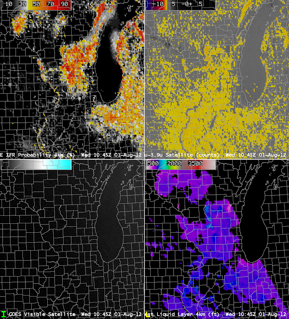
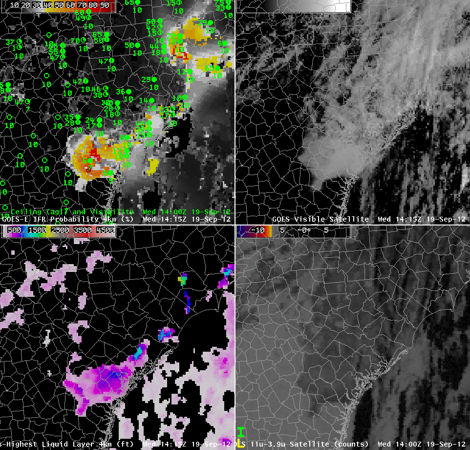
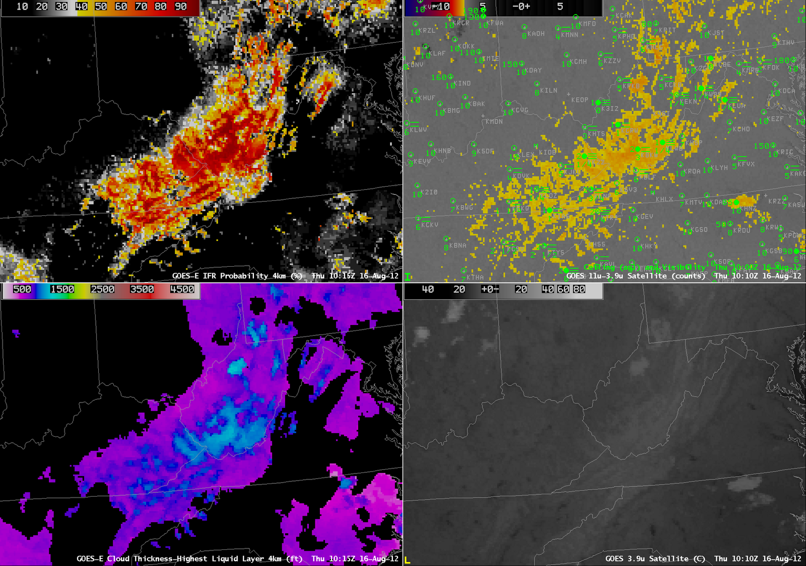
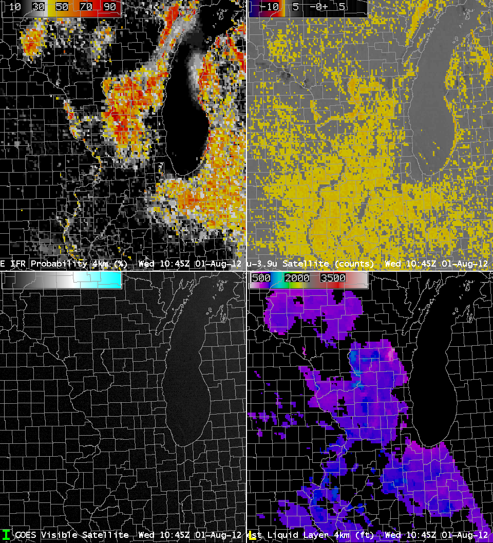
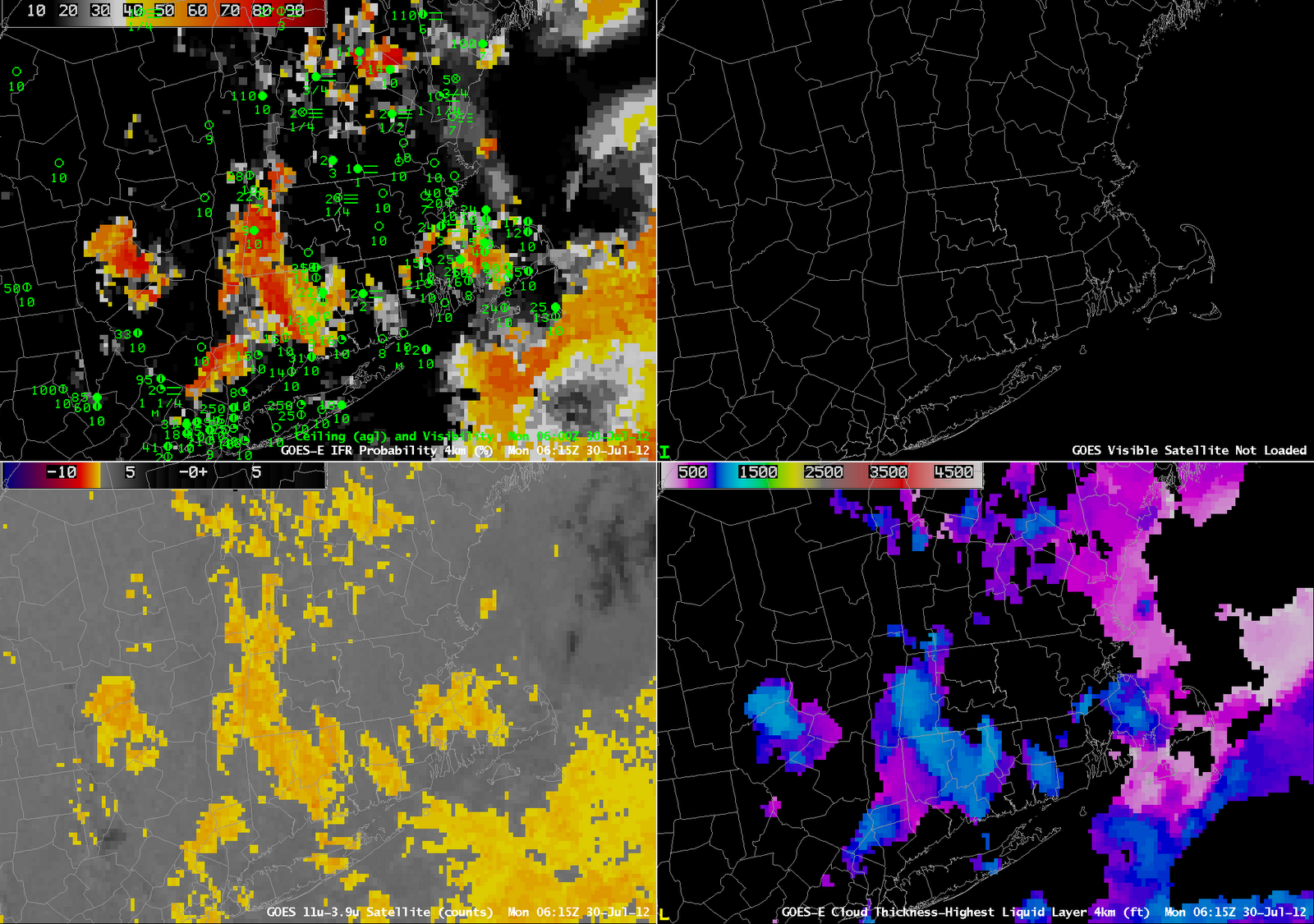
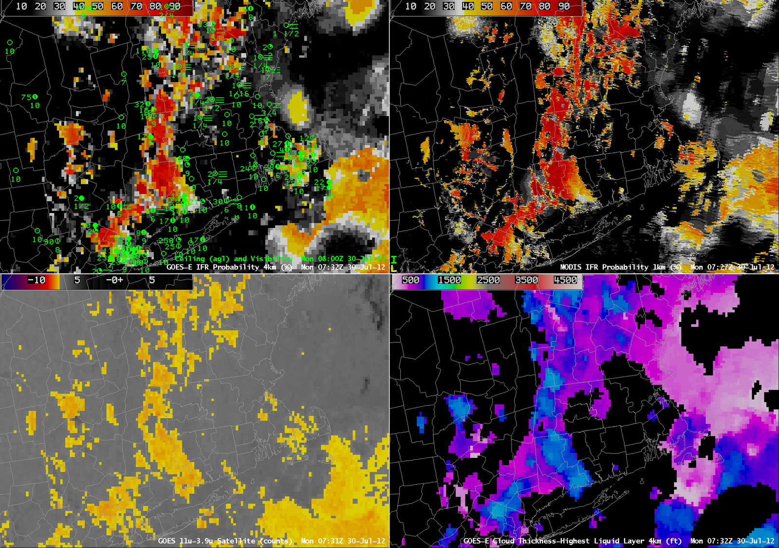
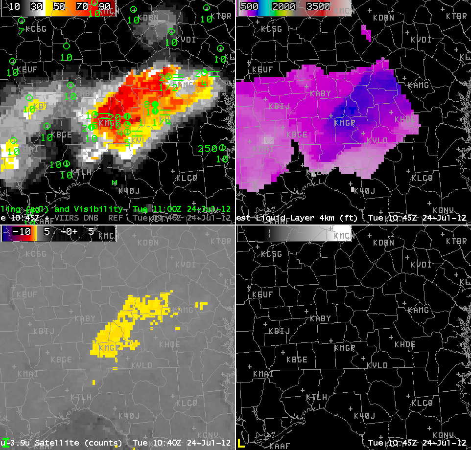
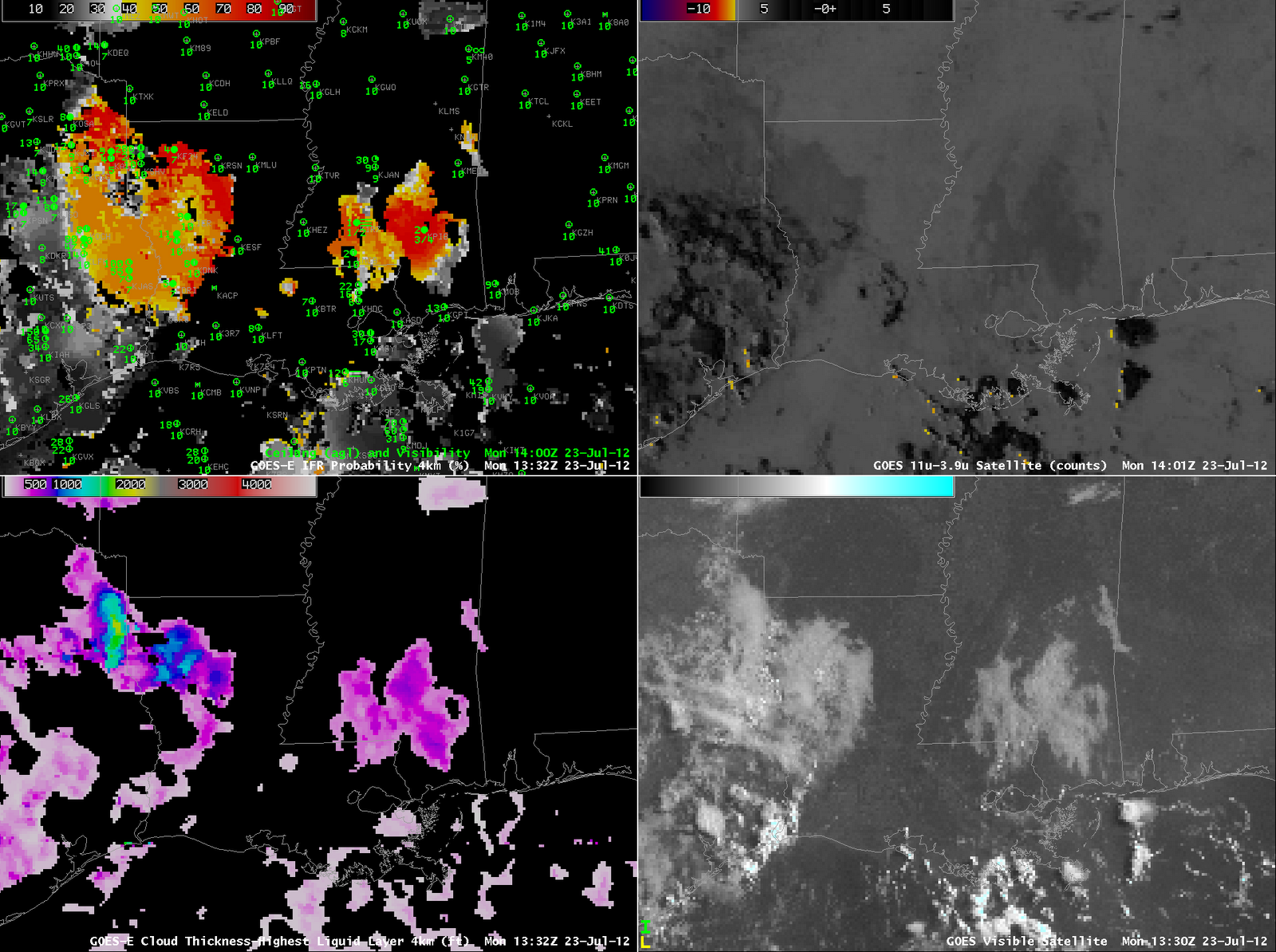
GOES-R IFR Probabilities (Upper Left), Traditional Brightness Temperature Difference Fog Product (upper right), Visible Imagery (lower left), GOES-R Cloud Thickness (lower right), all from 1045 UTC on 1 August 2012

Note that the IFR Probabilities (above, upper left) are highest over south-central Wisconsin.  In addition, a ribbon of higher values snakes down the Wisconsin River, and down the Mississippi River, in accordance with observations at 1232 UTC.  In contrast, the brightness temperature difference field shows returns suggestive of fog over most of Illinois and eastern Iowa, where fog was not observed just after sunrise.  The curious lack of fog signal over the Mississippi and Illinois Rivers likely arises from the co-registration error (discussed here) that also causes the spike in brightness temperature difference signal along the southeastern shore of Lake Michigan.

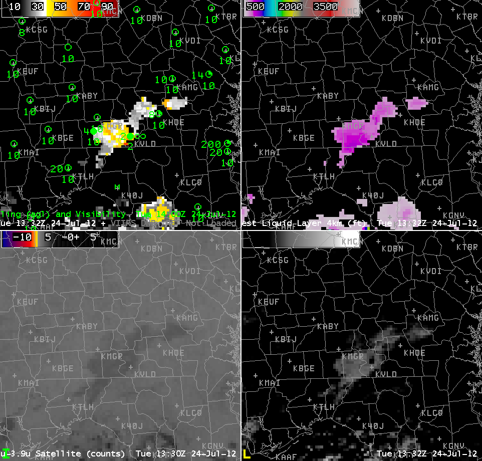
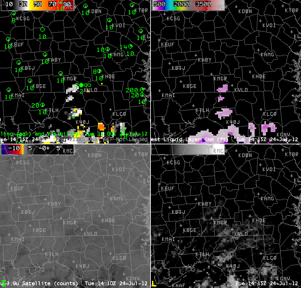
The thickest clouds are diagnosed at 1045 UTC (the last such image made before twilight conditions make the product unreliable) show the thickest clouds over central Wisconsin.  The 1415 UTC visible image, below, shows the region where fog/low clouds have lingered longest:  over central Wisconsin.

Visible Imagery from GOES-13, 1415 UTC on 1 August 2012

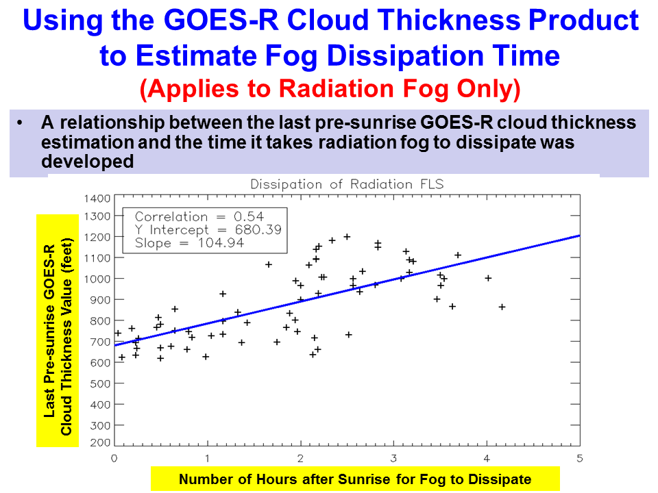
Again, GOES-R IFR Probabilities accurately outlined the region where fog was present (and equally importantly, where it was not).  The thickest clouds were the last to erode.  The relationship between fog thickness and dissipation time is given here.

Data from the GEOCAT browser at CIMSS shows how the GOES-R IFR Probabilities field evolved with time in the early morning hours of the 1st (below)

GOES-R Probabilities are too low: Why?

GOES-R IFR Probabilities (upper left), GOES-East Visible imagery (upper right), Brightness temperature difference between 10.7 and 3.9 micrometers (lower left), GOES-R Cloud Thickness (lower right)

The imagery above shows high IFR probabilities over western Massachusetts — where IFR conditions are not observed — and very low probabilities in central Massachusetts in and near the Connecticut River Valley where IFR conditions are observed.  The brightness temperature difference in central Massachusetts is not suggestive of low clouds and fog.  For the IFR probability to be high there, then, would require that the Rapid Refresh Model showed saturation in the lower part of the model atmosphere.  Thus, the fused product could show higher probabilities in this region where fog is observed.  However, as shown below, relative humidity in the lowest part of the model was actually a relative minimum over central Massachusetts.

Two-hour forecasts of Relative Humidity from the Rapid Refresh, all valid at 0600 UTC from the 0400 UTC model run;  Lowest 30 mb of the model (upper left), lowest 60 mb of the model (upper right), lower 90 mb of the model (lower left), surface (lower right)
Two-hour forecasts of Relative Humidity from the Rapid Refresh, all valid at 0800 UTC from the 0600 UTC model run;  Lowest 30 mb of the model (upper left), lowest 60 mb of the model (upper right), lower 90 mb of the model (lower left), surface (lower right)

By 0730 UTC, the satellite brightness temperature difference product (below) is starting to suggest that fog/low clouds are more widespread (A MODIS image at the same time tells the same tale).  As that happens, the IFR probabilities start to increase.

GOES-R IFR Probabilities computed from GOES-East imager data (upper left), GOES-R IFR probabilities computed from MODIS data (upper right), Brightness temperature difference between 10.7 and 3.9 micrometers (lower left), GOES-R Cloud Thickness (lower right)
GOES-R IFR Probabilities (upper left), GOES-East Visible imagery (upper right), Brightness temperature difference between 10.7 and 3.9 micrometers (lower left) at 1032 UTC, GOES-R Cloud Thickness (lower right) not shown because of twilight conditions

The 1032 UTC imagery (above) shows the very small scale of this fog feature that is in central Massachusetts.

Fog Dissipation

GOES-R IFR Probability (upper left), GOES-R Cloud Thickness of highest Liquid Cloud Layer (upper right), Traditional brightness temperature difference (lower left) and Visible Imagery (lower right) over southern Georgia and northern Florida near 1100 UTC on 24 July 2012

GOES-R Cloud thickness at the last valid time before sunrise (recall that Cloud Thickness is not available during twilight times) can be used as a predictor for where low clouds/fog (that formed via radiative processes) will linger longest after sunrise.  In the image above, the thickest cloud — about 1000 feet thick — is diagnosed to be near KMGR (Moultrie, GA).  It is in this area that the fog should be last to dissipate.  The relationship between cloud thickness and time to dissipate was derived from Spring-time observations and is shown in the plot below.  (You can download the figure here as a png or here as a pdf).

This figure, from the GOES-R Fog/Low Stratus Training developed for the National Weather Service, shows dissipation time after sunrise as a function of Cloud Thickness
GOES-R IFR Probability (upper left), GOES-R Cloud Thickness of highest Liquid Cloud Layer (upper right), Traditional brightness temperature difference (lower left) and Visible Imagery (lower right) over southern Georgia and northern Florida near 1330 UTC on 24 July 2012

The visible imagery shows that fog is lingering as expected in the region between Moultrie and KVLD (Valdosta).  By 1401 UTC, below, the fog has largely dissipated as cumulus convection starts to develop surrounding the region where fog had existed.

GOES-R IFR Probability (upper left), GOES-R Cloud Thickness of highest Liquid Cloud Layer (upper right), Traditional brightness temperature difference (lower left) and Visible Imagery (lower right) over southern Georgia and northern Florida near 1415 UTC on 24 July 2012

Fog over Louisiana and Mississippi

GOES-R IFR Probabilities computed from GOES-East Imager data (upper left), GOES-East brightness temperature difference (upper right), GOES-R Cloud Thickness of the highest liquid water cloud layer (bottom left), Suomi/NPP Day/Night band (bottom right), all from 0830-0900 UTC on 23 July 2012.
Enhanced 11-micrometer imagery, 0831 UTC 23 July 2012

Fog formed over the southern Mississippi Valley in the early morning of July 23 in a region where high clouds associated with a westward-tracking wave made detection difficult via the traditional brightness temperature difference method.  The imagery above shows relatively high IFR probabilities over southwestern Louisiana where IFR conditions are occurring.  Two items should jump out.  The IFR probabilities are highest where both satellite and model predictors are high, and that occurs in west-central Louisiana.  In regions to the south and west, where higher clouds exist (and satellite predictors are therefore low), probabilities are a bit lower in a region where only model predictors are being used.  However, IFR conditions are present.  Note how the character of the IFR probability field changes from the region where satellite data are used (much more spatially variable) to the region where mostly model data are used (more spatially uniform).  It is very important when interpreting the probability fields to be aware of the presence of high clouds that limit the inclusion of satellite data in the predictors.

GOES-R IFR Probabilities computed from GOES-East Imager data (upper left), GOES-East brightness temperature difference (upper right), GOES-R Cloud Thickness of the highest liquid water cloud layer (bottom left), Suomi/NPP Day/Night band (bottom right), all from 1145-1200 UTC on 23 July 2012.
GOES-R IFR Probabilities computed from GOES-East Imager data (upper left), GOES-East brightness temperature difference (upper right), GOES-R Cloud Thickness of the highest liquid water cloud layer (bottom left), Suomi/NPP Day/Night band (bottom right), all from 1215 UTC on 23 July 2012.

The two images above show how the probabilities change as the predictors used change from nighttime values (at 1145 UTC) to daytime values (1215 UTC).  At 1145 UTC, probabilities over Louisiana are near 40%, and these probabilities are driven largely by model data, because of high clouds.  There are several airports reporting IFR conditions at 1200 UTC.  Probabilities jump to around 55% at 1215 UTC.

GOES-R IFR Probabilities computed from GOES-East Imager data (upper left), GOES-East brightness temperature difference (upper right), GOES-R Cloud Thickness of the highest liquid water cloud layer (bottom left), GOES-East Visible imagery (bottom right), all from around 1300 UTC on 23 July 2012.

At 1300/1400 UTC, the GOES-R IFR probabilities and cloudt thickness fields neatly overlap the visible imagery observations of cloudiness over Mississippi and over western Louisiana, with a pronounced break in central Louisiana.

Terrain

GOES-R IFR Probabilities (Upper left), GOES-R Cloud Thickness (Upper right), Terrain with surface plots of Ceiling (above MSL) and visibility (lower left) and the GOES-15/GOES-13 Water vapor imagery

When terrain rises up into the clouds, IFR conditions occur, and the GOES-R IFR product shows that effect.  These images from ~1200 UTC on 19 July 2012 show two regions of IFR conditions over the Pacific Northwest — along the spine of the coastal range from the Olympic Mountains south to the Oregon Coast Range and along the Cascades from east of Seattle southward to Oregon.  The observations shown in the lower left (with ceilings above mean sea level, plotted over topography) are consistent with the IFR probabilities:  Low probability over the region between the coastal range and the Cascades, and high probability in regions over the Cascades where the height exceeds the observed ceilings over, say, Seattle and Portland, and high probabilities along the Coastal Range where heights exceed the observed ceilings along the coast.