Category Archives: Cloud Thickness

Low Clouds over the Florida Peninsula

GOES-R IFR Probability computed from GOES-East and Rapid Refresh data (Upper left), Traditional Brightness Temperature Difference (10.7 µm – 3.9 µm) Product from GOES (Upper right), GOES-R Cloud Thickness product (Lower Left), Brightness Temperature Difference (10.8 µm – 3.74 µm) Product from VIIRS on Suomi/NPP (Lower Right)

Tuesday morning’s low cloud/fog event over southern Florida is an excellent example of how the fused product better distinguishes between fog (that reduces visibility at the surface) and low stratus (that does not reduce visibility at the surface).  The traditional brightness temperature difference products from both GOES (Upper Right) and VIIRS (Lower Right) show a strong signal over both Florida coasts — Atlantic and Gulf — but the IFR probabilities are highest along the Atlantic Coast — where IFR and near-IFR ceilings/visibilities are observed.  Over and off the west coast of Florida, despite the very strong satellite signal, IFR probabilities are low because saturation is not occurring in the lowest part of the Rapid Refresh Model — and IFR conditions are not observed.

IFR Conditions over Southwest Alaska

GOES-R IFR Probabilities computed using GOES-West and Rapid Refresh Data (Upper Left), GOES-R Cloud Thickness (Upper Right), GOES-West Brightness Temperature Difference (10.7 µm – 3.9 µm) (Lower Left), Topography over Southwest Alaska (Lower Right).

(Stations discussed below:  Bethel (PABE) and McGrath (PAMC) on the Kuskokwim River, Sparrevohn Air Force Base (PASV), Dillingham (PADL), Cape Newehnam Air Force Base (PAEH) and St. Marys (PASM) on the Yukon River)

Portions of Southwestern Alaska in the Kuskokwim and Yukon River valleys experienced IFR or near-IFR conditions overnight between 11 and 12 November.  How did the half-hourly animations of GOES-R IFR probability and cloud thickness (as well as the traditional brightness temperature difference product) depict those reduced visibilities?

The beginning of this animation shows the effect of twilight conditions on the Cloud Thickness Product (upper right);  this product shows the thickness of the highest boundary layer cloud during non-twilight conditions.  If twilight conditions are occurring, or if higher clouds are moving into a region (as is occurring over Nushagak and Bristol Bays near Dillingham at the end of the animation), then the product is not generated.

The area of IFR conditions over southwest Alaska from St. Marys to Sparrevohn, McGrath and Bethel southwestward to Dillingham is depicted will in the IFR Probability fields.  Light winds in this region are allowing the low clouds to develop.  Relatively high values of IFR Probabilities, and the pixelated look to the field mean that both satellite and model predictors are being used over most of this region in computing the IFR probabilities.  An exception occurs over Cape Newenham near the end of the animation when lower IFR probabilities and a smoother field suggest that satellite-based predictors are not being used (because of the presence of multiple cloud layers).  This is also true of regions in the far southwestern part of the shown domain at the end of the animation.

IFR Conditions under Cirrus in Florida

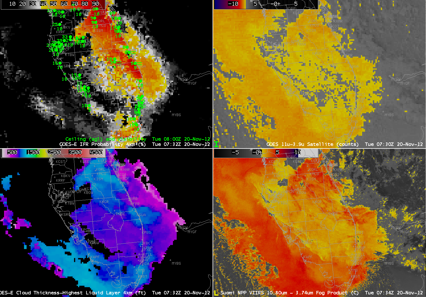
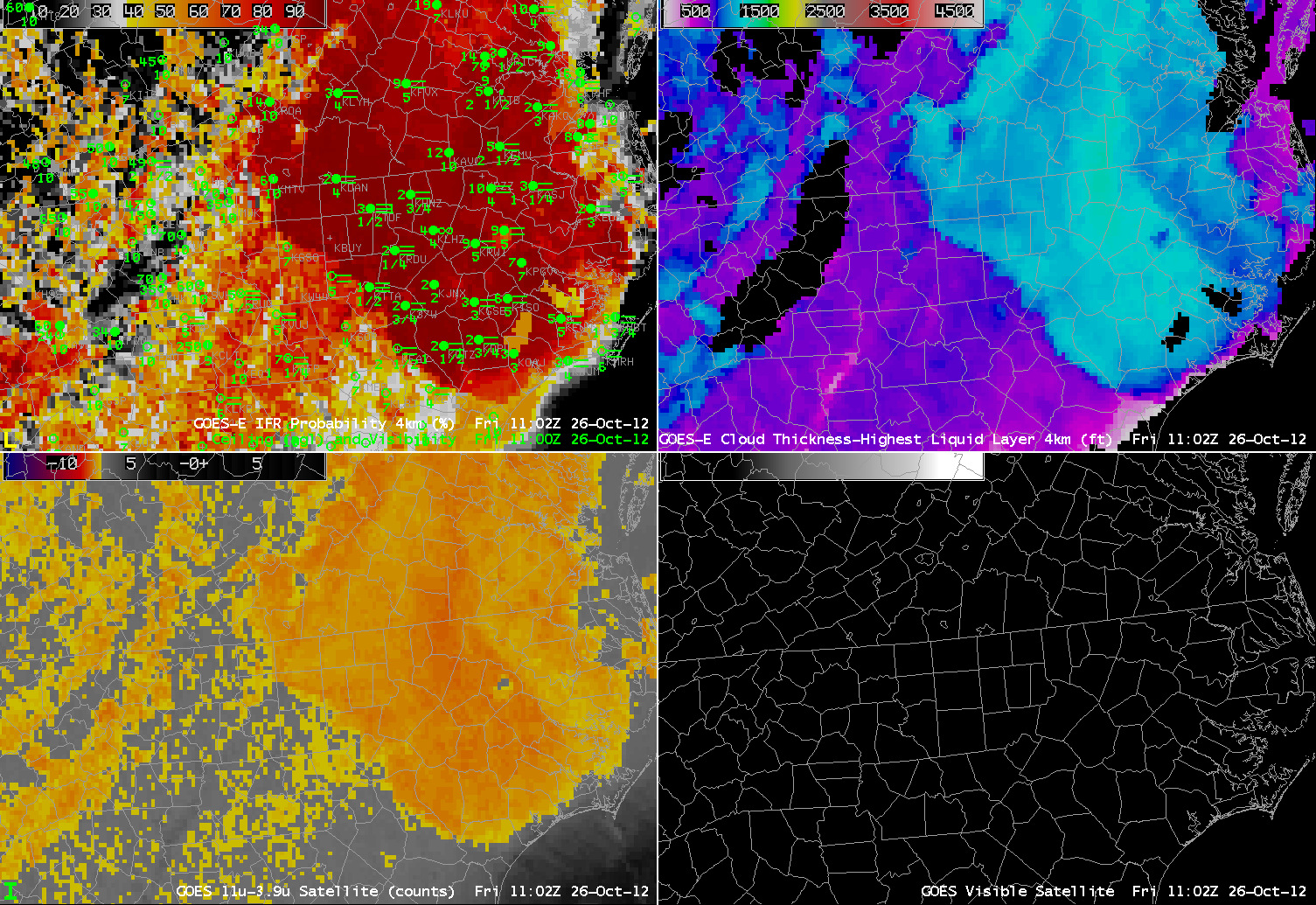
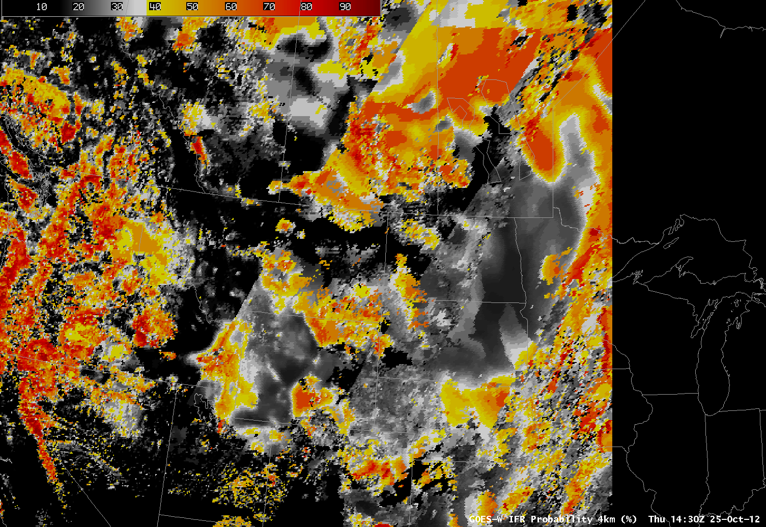
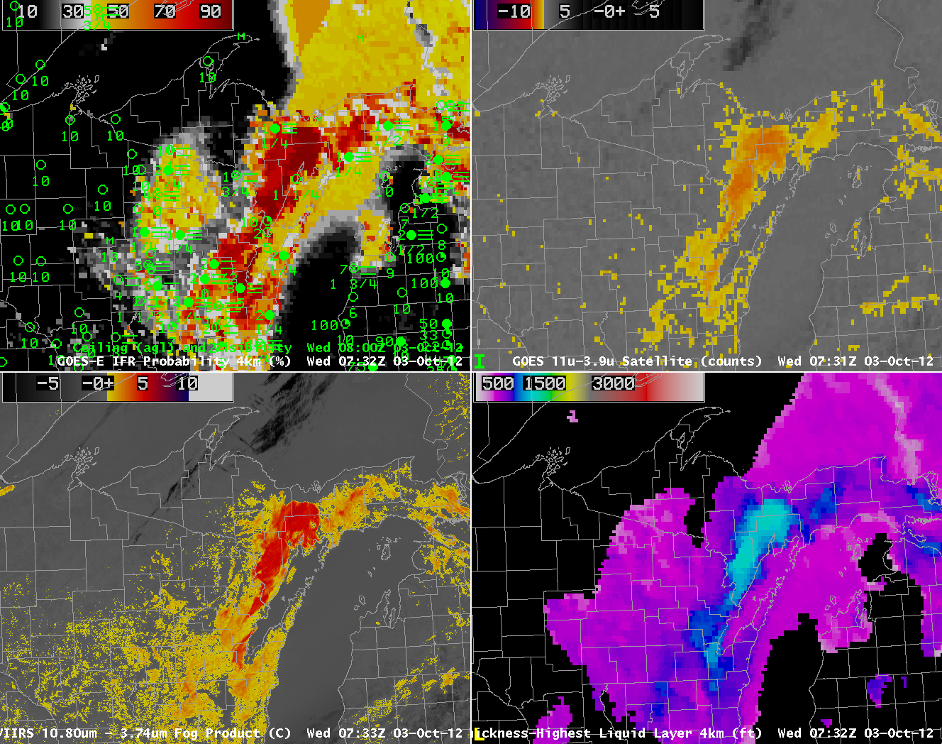
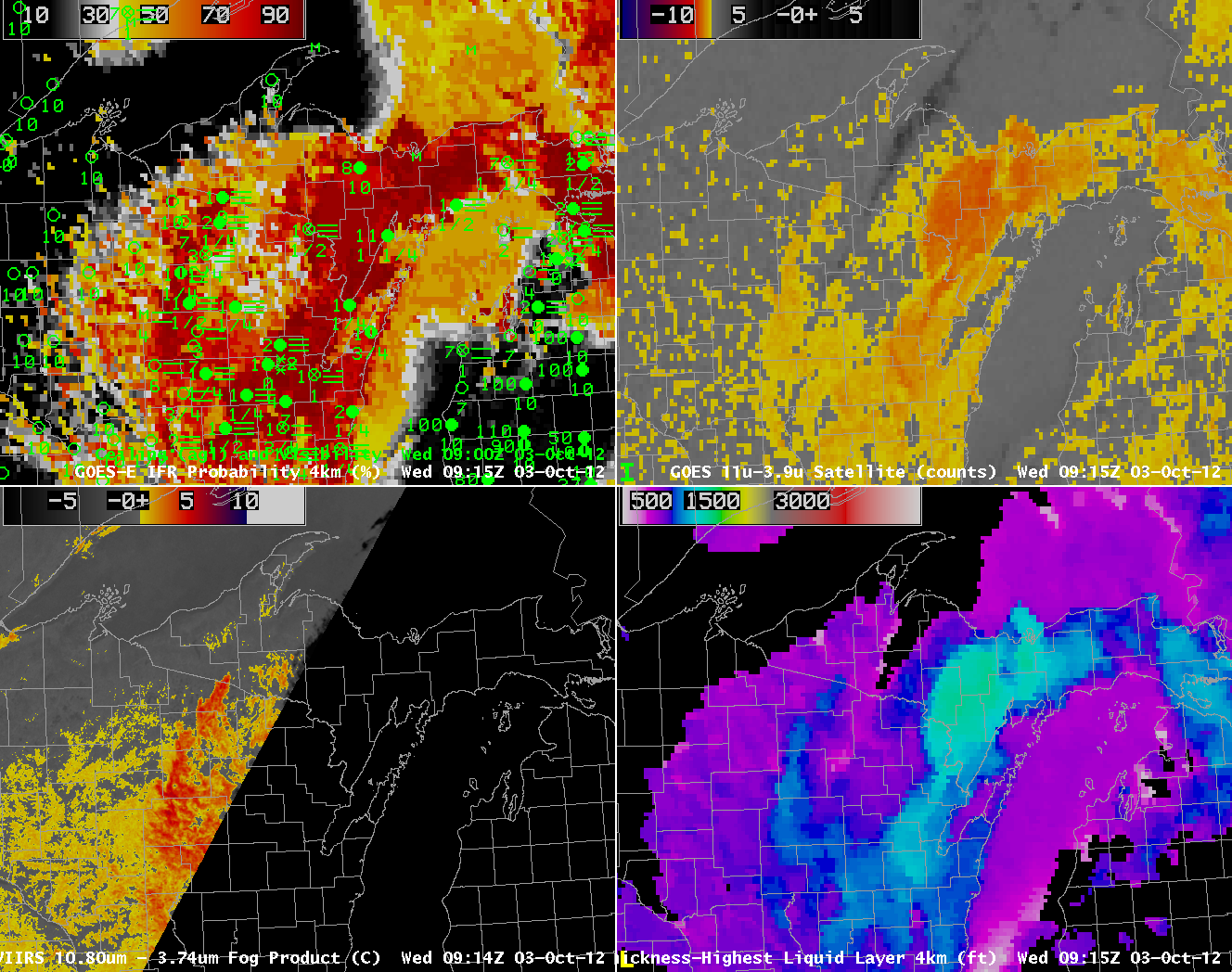
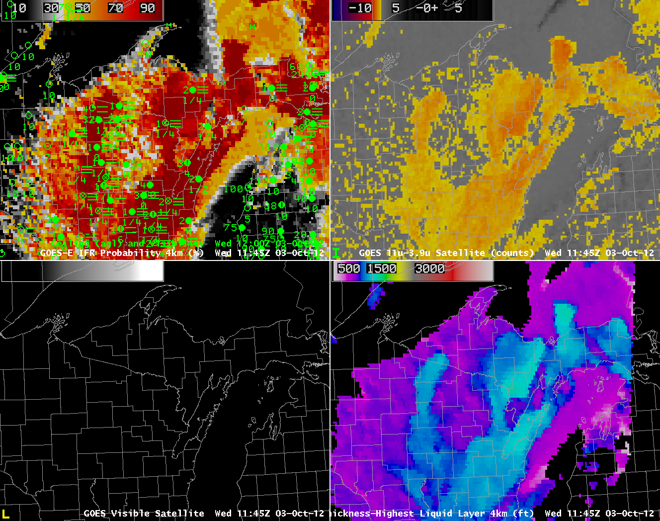
GOES-R IFR Probabilities from GOES-East (Upper Right), GOES-East traditional ‘fog product’ (Brightness Temperature Difference 10.7 µm – 3.9 µm), GOES-R Cloud Thickness, GOES-East Water Vapor (6.5 µm) imagery

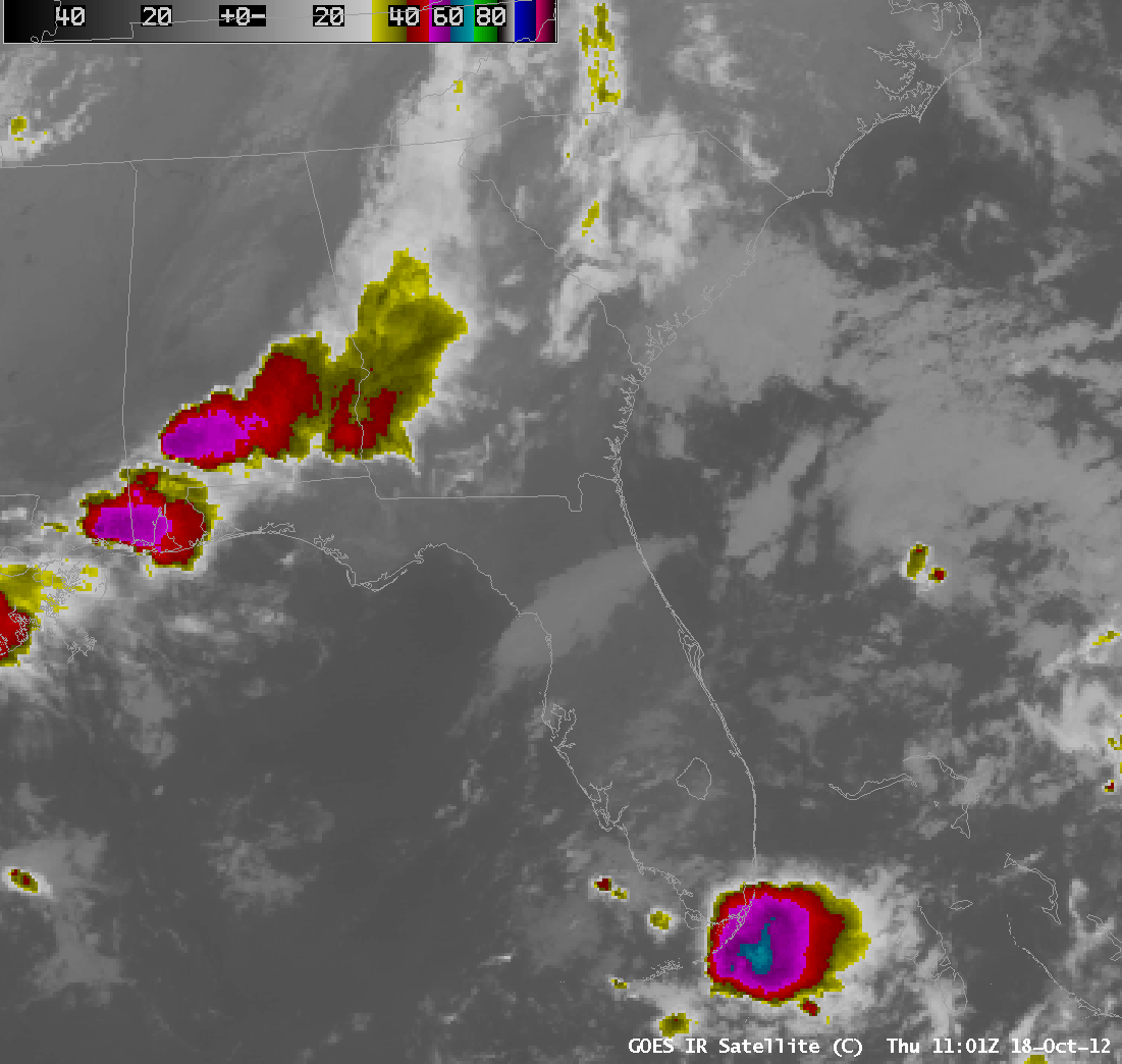
Fog developed over central Florida overnight underneath a thin cirrus (as indicated by both the water vapor and brightness temperature difference imagery).  Cirrus clouds prevent the traditional brightness temperature difference field from identifying low fog/stratus because the high ice clouds are detected rather than the developing low-level water clouds.  This is a case, then, when a fused product gives needed surface information to help diagnose the development of fog and low stratus.  The brightness temperature difference product, the traditional method to detect fog and low stratus, is giving no information where dense fog is forming.

On this date, the development and expansion of the higher IFR probabilities over central Florida neatly matches the development of IFR conditions at the observing stations.  Probabilities are not high because the satellite predictors are not contributing to the algorithm.  It is important when interpreting the IFR probabilities to be aware of the presence of high clouds that will influence IFR probability values.  Where the cirrus clouds are not present, notably over northeast Florida, IFR probabilities are much higher because satellite predictors there are contributing to the final probability.

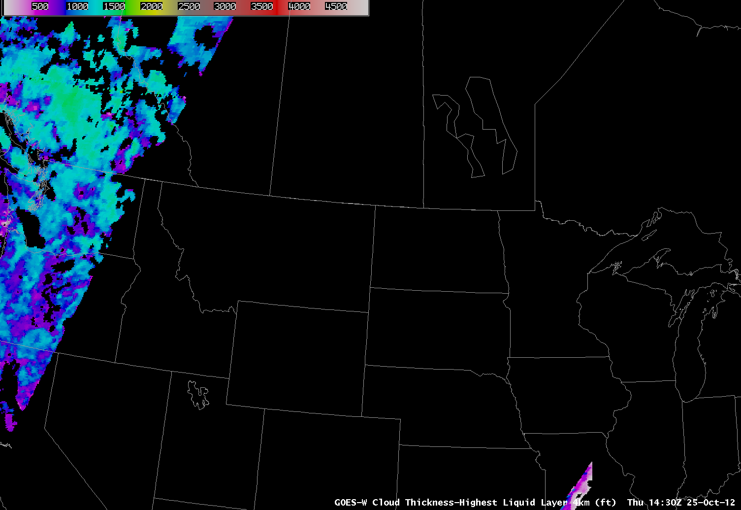
This case also shows that the Cloud Thickness is only computed where the highest clouds detected is a water-based cloud.  Underneath the cirrus shield, except for a few regions where there are apparently holes, cloud thickness is not computed.

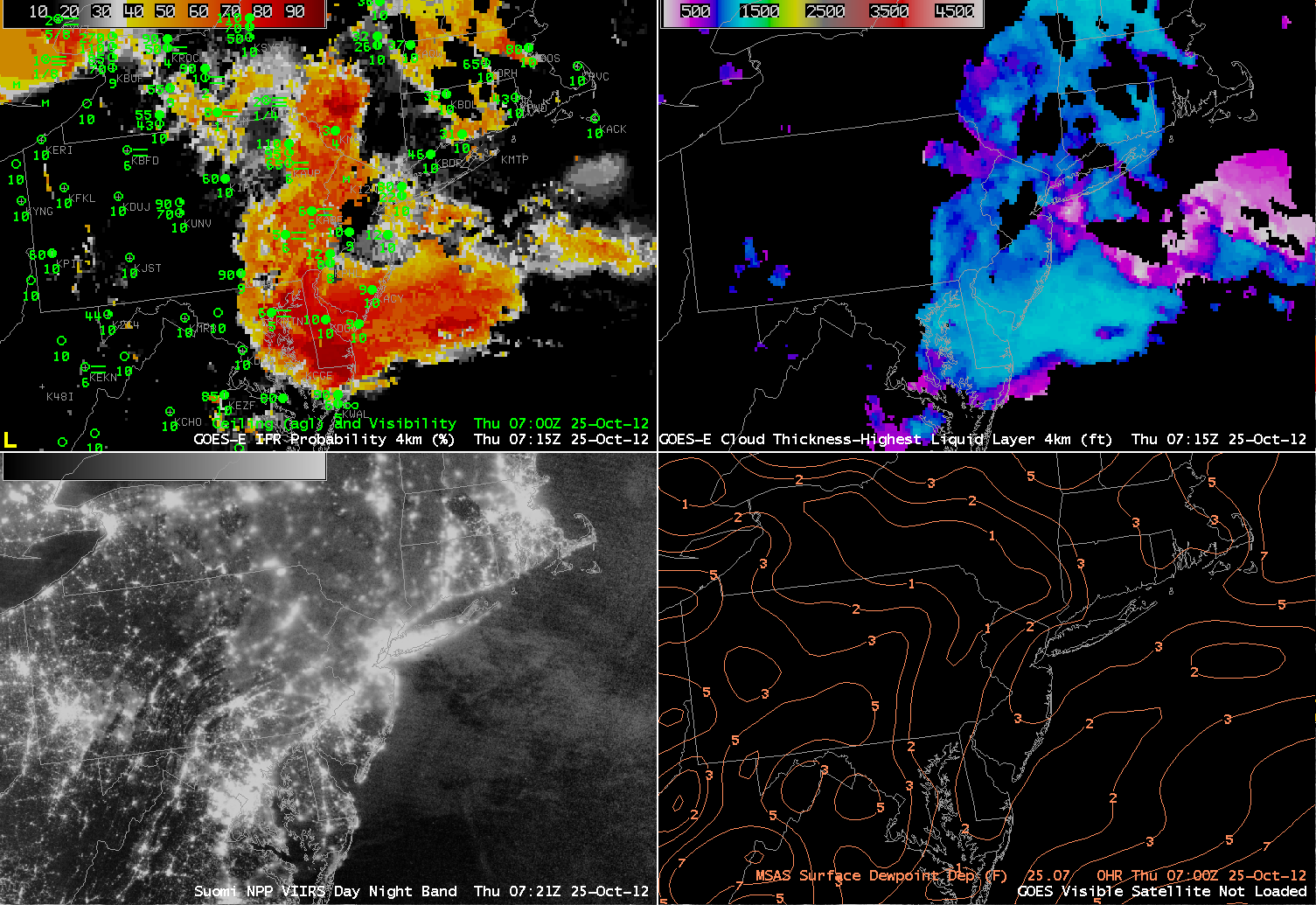
GOES-R IFR Probabilities and Day/Night Band from VIIRS on Suomi/NPP, 0715 UTC 5 Nov

The toggle above flips between the Day-Night band from VIIRS on Suomi/NPP and the GOES-R IFR probability at the same time.  The thin cirrus shield is readily apparent, and the regions of fog are also visible in the Day/Night band over north-central Florida and over coastal South Carolina.

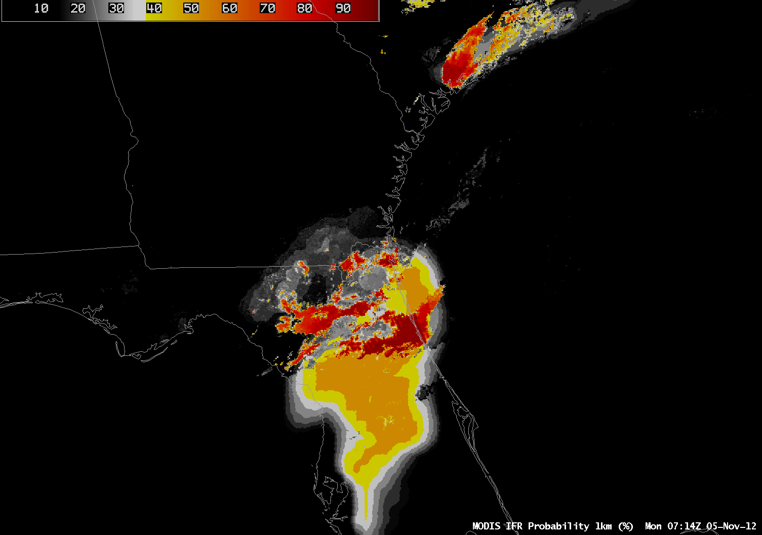
A MODIS-based IFR Probability (shown below) was also created at 0715 UTC, and it shows a pattern similar to that above.  The pixelated part of the image corresponds to where satellite data are being used.  The region with lower values, and a flatter field, was created using only model predictors and, as noted above, is characterized by lower probabilities.  The highest probabilities are in regions where both satellite and model predictors are very confident that IFR conditions are present.

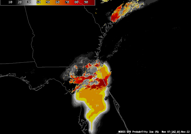
MODIS-based GOES-R IFR Probabilities, Monday 5 Nov 2012, 0714 UTC

Stratus vs. Fog in Montana/North Dakota

Suomi/NPP VIIRS Day/Night Band Visible imager (upper left), Traditional Brightness Temperature Difference (10.7 µm – 3.9 µm) image (upper right), GOES-R Cloud thickness algorithm (lower left), GOES-R IFR Probability (lower right)

Both the nighttime visible image from the Suomi/NPP VIIRS instrument (which uses moonlight as an illumination source) and the traditional brightness temperature difference product suggest the presence of water-based clouds over eastern Montana and northwest North Dakota on the morning of 31 October 2012.  However, there are no reports in Montana of IFR conditions.  GOES-R IFR Probabilities overlapping the cloud deck are very low.  It is likely that this cloud feature is elevated stratus, and that saturation is not occuring in the lowest levels of the model.  Fusing both model and satellite data yields a product that can be greater than the sum of the two.  Note, however, the IFR conditions that do exist in Bismarck, where IFR probabilities are very low and satellite information shows no fog signal.  This is likely very small scale river fog in the Missouri River Valley that is both too small to be resolved in the model or detected by the satellite.  In addition, very thin cirrus is interfering with the detection of low-level water clouds in much of central North Dakota.

Marine Stratus, Day 2

GOES-R IFR Probability (Upper Left), GOES-R Cloud Thickness (Upper Right), GOES-East Brightness Temperature Difference (10.8 µm – 3.9 µm) (Lower Left), GOES-East Visible Imagery (Lower Right) at 0800 UTC 26 October 2012

The marine stratus over the mid-atlantic on Oct 25th (Link) has continued to spread southwestward into North Carolina, and higher values in the IFR probability fields continue to overlap nicely with observed IFR conditions in the Piedmont of North Carolina.  The image above at 0800 UTC, and below at 1100 UTC, show deteriorating flight conditions as the high probabilities ooze southwestward.  Note that the traditional brightness temperature difference field does show a signature of the cirrus outflow from Hurricane Sandy off the coast of the Carolinas, in the extreme southeast part of the images, both at 0800 UTC and 1100 UTC.

GOES-R IFR Probability (Upper Left), GOES-R Cloud Thickness (Upper Right), GOES-East Brightness Temperature Difference (10.8 µm – 3.9 µm) Lower Left), GOES-East Visible Imagery (Lower Right) at 1100 UTC 26 October 2012
GOES-R IFR Probability (Upper Left), GOES-R Cloud Thickness (Upper Right), GOES-East Brightness Temperature Difference (10.8 µm – 3.9 µm) Lower Left), GOES-East Visible Imagery (Lower Right) at 1600 UTC 26 October 2012

By 1600 UTC, the cirrus canopy from Sandy has overspread most of eastern North Carolina.  This makes satellite data less useful in computing IFR probabilities, and Model Data comparatively more important, and the character of the IFR probability field does change, with a smoother field overall.  At 1600 UTC the probabilities have decreased; the temporal evolution of the field (not shown) is still giving important information, especially in concert with the surface visibility/ceiling observations.  The decrease in probabilities is gradual as the Sun slowly works to warm the boundary layer.

Day/Night Transition artifacts

GOES-R IFR Probability, 1430 UTC on 25 October 2012

The predictors used by the GOES-R IFR Probability algorithms change as night turns to day and vice versa.  For example, the daytime predictors include the visible satellite imagery.  The change in predictors occurs when the solar zenith angle is less than 85 degrees (that is, when the sun is just rising). For solar angles between 85-90 degrees, temporal continuity has an increased importance and therefore the IFR probabilities look very similar to the previous temporal images.  When the solar zenith angle is between 80-85 degrees temporal metrics are used combined with current visible channel data (only if certain tests are passed that prove the data is of good quality). The cloud mask sometimes has difficulty detecting low clouds in this region so it still is not fully utilized until the solar zenith angle drops to below 80 degrees, where the cloud mask and the full array of daytime predictors are used. This leads to discernible changes in the probability fields, as shown above.  Two boundaries, extending southwest to northeast (roughly parallel to the terminator) are apparent, one from extreme northwest Utah through central Montana and into Canada (where the solar angle is around 85 degrees) and one from northwest Colorado through northwest South Dakota into Manitoba (where the solar angle increases above 80 degrees).   This transition zone is less noticeable in the Summer because of the Earth-Sun geometry.  It is very difficult to create the GOES-R Cloud Thickness product when the solar zenith angles are between 75-90 degrees so the product is currently not available in this region.  This is why the Cloud Thicknesses cut off over eastern Oregon and show back up over central Missouri.

GOES-R Cloud Thickness for 1430 UTC, 25 October 2012

Marine Stratus in the Mid-Atlantic States

GOES-R IFR Probabilities computed from GOES-East (upper left), GOES-R Cloud Thickness in ft (upper right), Brightness Temperature Difference (10.8 µm – 3.74 µm) computed from Suomi/NPP VIIRS data, Brightness Temperature Difference (10.8 µm– 3.9 µm) computed from GOES East, all valid about 0700 UTC 25 October 2012

Marine Stratus has moved inland over Maryland and surrounding states overnight, and the GOES-R IFR probabilities capture the visibility restrictions that have accompanied it.  The imagery above includes the traditional brightness temperature difference fields computed from Suomi/NPP (horizontal resolution:  1 km at nadir) and from GOES (nominal horizontal resolution:  4 km at nadir).  The distinct leading edge of the marine layer is readily apparent in the Susquehanna River Valley.  Note, however, that the strong returns over the Hudson River Valley do not correlate well with reduced visibilities. The GOES-R IFR probabilities do a good job depicting the marine layer in the Susquehanna River Valley (shown by the relatively high probabilities), but return much lower probabilities over the Hudson River Valley where surface observations indicate hazardous low clouds are not present.  Again, this is a benefit of using a fused product.

GOES-R IFR Probabilities (Upper Left) and Cloud Thickness (Upper Right), Suomi/NPP Day/Night Band (Lower left) and MSAS-derived Dewpoint depression on top of Visible imagery.  Times as indicated

The temporal resolution of GOES-R IFR products allow for continuous monitoring of an evolving situation, making up for the relatively poor horizontal resolution (compared to polar orbiting platforms like Suomi/NPP or Terra/Aqua).  The IFR probability field neatly captured the relentless inland push of the marine stratus air, and as the probabilities increase at locations, IFR conditions become more likely.  The loop above includes a Day/Night band image that is reproduced below.  The day/night band, even in low lunar light cases, can distinguish between clear sky and clouds over ocean.  Over land, however, the interpretation is complicated by city lights shining through clouds.  Nevertheless, the cloudy region can be discerned over parts of eastern Pennsylvania and Maryland, where the light signal is more diffuse.

Fog/Low stratus in California

GOES-R IFR Probabilities (Upper left) and GOES-15 brightness temperature difference (10.7 µm – 3.9 µm) (upper right) from 0200 UTC

 GOES-R IFR Probabilities can be used to evaluate and monitor the evolution of marine stratus as it (nightly) moves inland from the Pacific Ocean to adjacent land over California, as well as the evolution of fog and low clouds/haze over the central Valley of California.  At 0200 UTC — near sunset — as shown above, IFR conditions are diagnosed from fused satellite and model data to be most likely offshore, despite a brightness temperature difference signal in California’s Central Valley, where airports are not reporting IFR conditions.  In other words, the GOES-R IFR algorithm is correctly suppressing the satellite signal inland.

GOES-R IFR Probabilities (Upper left) and GOES-15 brightness temperature difference (10.7 µm – 3.9 µm) (upper right) from 0700 UTC

 By 0700 UTC, ceilings and visibilities in the Salinas and Central Valleys have started to lower as IFR probabilities decrease.

GOES-R IFR Probabilities (Upper left) and GOES-15 brightness temperature difference (10.7 µm – 3.9 µm) (upper right) from 0900 UTC, Suomi NPP Brightness Temperature Difference (10.8 µm – 3.74 µm) (lower left)

 Ceilings and visibilities decrease further by 0900 UTC, as shown above.  Reasons for the difficulty in accurately diagnosing the probabilities over the Salinas Valley can be inferred from the figure above, which includes a (high-resolution) Suomi/NPP Brightness temperature difference plot that has a strong signal all along the Salinas Valley; such a strong signal is not so evident in the GOES brightness temperature difference field that uses data at coarser resolution.  It’s important that the satellite signal is strong in this fused product because the valley is not well-resolved in the Rapid Refresh Model.  When GOES-R is operational, infrared resolution will be 2 km — in between that of Suomi/NPP (1 km) and GOES (4 km).

GOES-R IFR Probabilities (Upper left) and GOES-15 brightness temperature difference (10.7 µm – 3.9 µm) (upper right) from 1400 UTC, GOES-R Cloud Thickness (lower left)

 The 1400 UTC image includes cloud thickness as diagnosed by the GOES-R algorithm.  Cloud thickness is well correlated with dissipation time for radiation fog — but not necessarily for advection fog.  Nevertheless, the regions diagnosed with thickest fog above continue to show fog in the visible imagery below, from 1600 UTC.

GOES-R IFR Probabilities (Upper left) and GOES-15 brightness temperature difference (10.7 µm – 3.9 µm) (upper right) from 1400 UTC, GOES-15 Visible Imagery (lower left)

Fog Over Florida

GOES-R IFR Probabilities (from GOES-14 and GOES-13) (upper left), Thickness of lowest liquid water cloud (upper right), Brightness temperature difference product from AVHRR (lower left), Brightness temperature difference product from GOES-East (lower right)

Light winds allowed for the development of radiation fog over Florida early in the morning of Oct 18th, 2012, and the GOES-R IFR Probability fields matched the development of the fog, with probabilities increasing over the course of the night as IFR conditions became more and more widespread.  The GOES-R IFR Probability product fuses satellite data with Rapid Refresh model output (as well as ancillary data such as SSTs and surface emissivity).

An interesting aspect of this case is the development of a mid-level cloud deck — visible in the AVHRR brightness temperature difference field at 1031 UTC (and in the GOES-R cloud thickness product as well, from GOES) over the north-central part of the Florida Peninsula.  A still image of the 10.7 micron field, below, plainly shows this mid-level feature.  This region of mid-level clouds correlates well with a slight drop in the GOES-R IFR probabilities.

GOES-14 10.7 micron imagery, 1101 UTC.

The Thickness of the lowest liquid cloud layer, upper right, can be correlated with fog dissipation time.  The last image before twilight conditions, at 1115/1132 UTC, shows thicknesses peaking around 1000 ft.  This corresponds to a dissipation time of at most 4 hours.  Indeed, a visible image at 1415 UTC show that the fog has largely dissipated.  The visibility at KJAX increases to 3 statute miles at 1419 UTC.

GOES-14 visible imagery at 1415 UTC on 18 October 2012

FLS detection over the upper midwest

0730 UTC GOES-R IFR Probabilities computed from GOES-14 (Upper left), Traditional Brightness Temperature difference (10.7 µm – 3.9 µm) from GOES-14 (Upper Right), Brightness Temperature Difference (11.35 µm – 3.74 µm) from VIIRS on Suomi/NPP (Lower left),  Thickness of highest Liquid Water Cloud Layer (Lower Right)

Low cloud formation over northern and northeastern Wisconsin early in the morning of October 3rd 2012 demonstrated some strengths of the fused GOES-R Fog/Low Stratus product.  Note that the 0732 UTC GOES-R IFR Probability has a pocket of higher probabilityes over north-central Wisconsin (near Vilas and Oneida Counties) in a region where the traditional brightness temperature difference has a weak signal, and in a region where surface observations indicate fog is present. This region is a good example of how the model RH data can amplify weak satellite signals where fog/low clouds are present but the satellite signal alone may not be strong enough to detect it.

0915 UTC GOES-R IFR Probabilities computed from GOES-14 (Upper left), Traditional Brightness Temperature difference (10.7 µm – 3.9 µm) from GOES-14 (Upper Right), Brightness Temperature Difference (11.35 µm – 3.74 µm) from VIIRS on Suomi/NPP (Lower left),  Thickness Of highest Liquid Water Cloud Layer (Lower Right)

At 0915 UTC, the region of IFR conditions in north-central Wisconsin persists.  At this time, however, the satellite signal also increases showing a signature consistent with low clouds/fog, and therefore GOES-R IFR probabilities significantly increase.  Two things should be clear.  First, the GOES-R IFR probability predicted the presence of Fog/Low Stratus before satellite signal was strong enough to detect it alone (a benefit of using a fused data product) and could be used better to nowcast the evolving boundary layer.  Second,  GOES-R IFR Probabilities when the model signal (in this case, the Rapid Refresh) is strong and the satellite signal is weak are lower than when both model and satellite signals are strong.  This is always the case.

1145 UTC GOES-R IFR Probabilities computed from GOES-14 (Upper left), Traditional Brightness Temperature difference (10.7 µm – 3.9 µm) from GOES-14 (Upper Right), Visible Imagery (0.62 µm) from GOES-14 (Lower left),  Thickness Of highest Liquid Water Cloud Layer (Lower Right)

The 1145 UTC shows the last pre-dawn estimate of Cloud Thickness over north-central Wisconsin (the terminator is apparent, running north-south through the Straits of Mackinac).  Estimated cloud thickesses over Vilas and Oneida counties are between 1000 and 1150 feet, vs. 1250 feet over Green Bay and more than 1300 feet over southern Upper Michigan.  Predictably, then, the fog/low stratus over north-central Wisconsin dissipates before the fog/low stratus over northeast Wisconsin and eastern Upper Michigan (see below).

1602 UTC GOES-R IFR Probabilities computed from GOES-14 (Upper left), Traditional Brightness Temperature difference (10.7 µm – 3.9 µm) from GOES-14 (Upper Right), Visible Imagery (0.62 µm) from GOES-14 (Lower left),  Thickness Of highest Liquid Water Cloud Layer (Lower Right)