 |
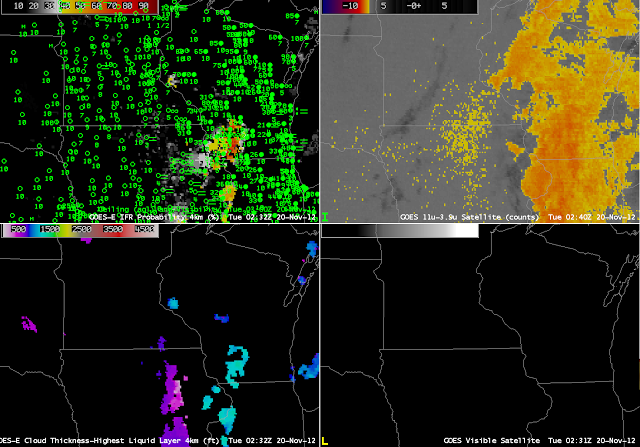
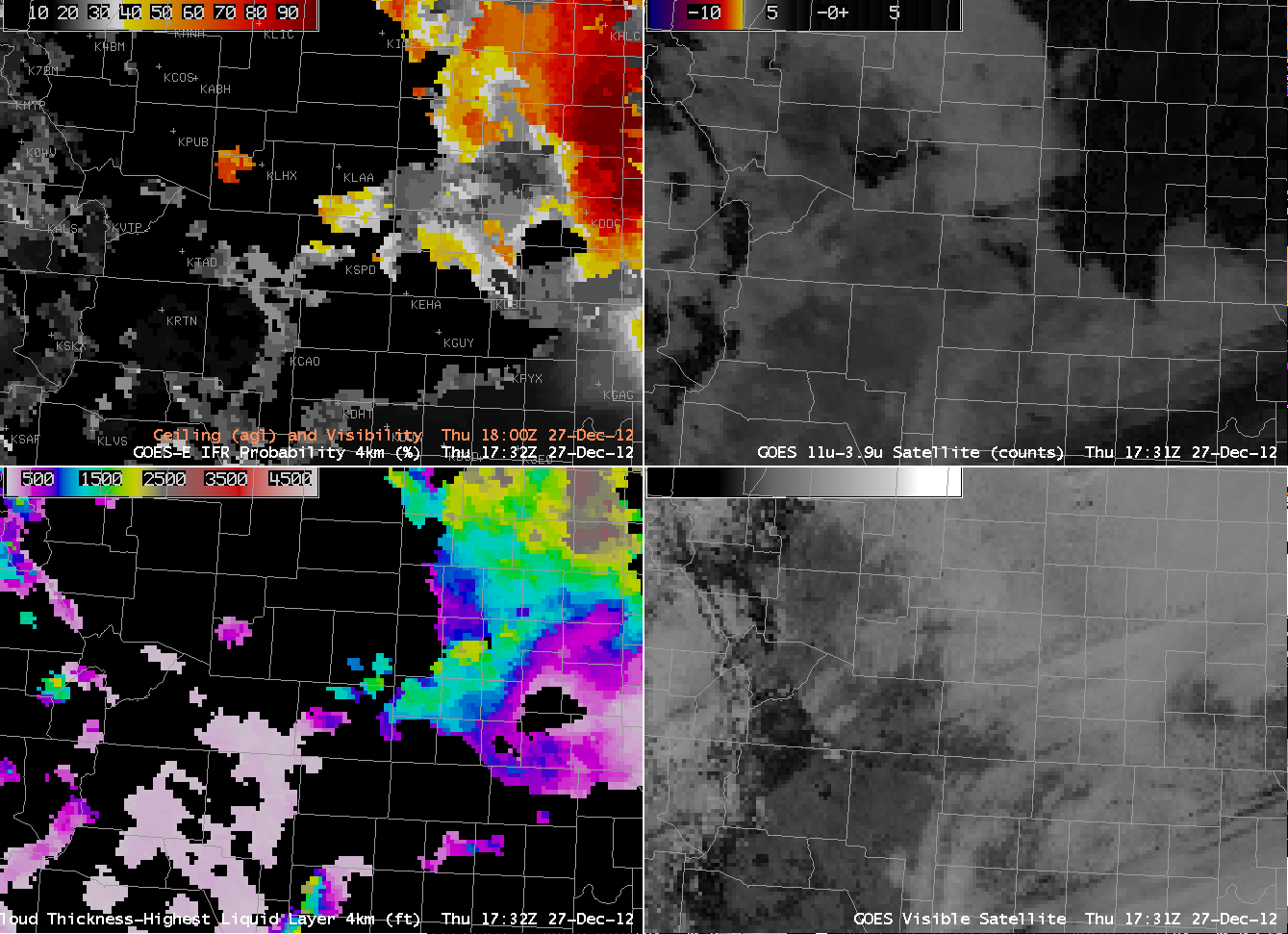
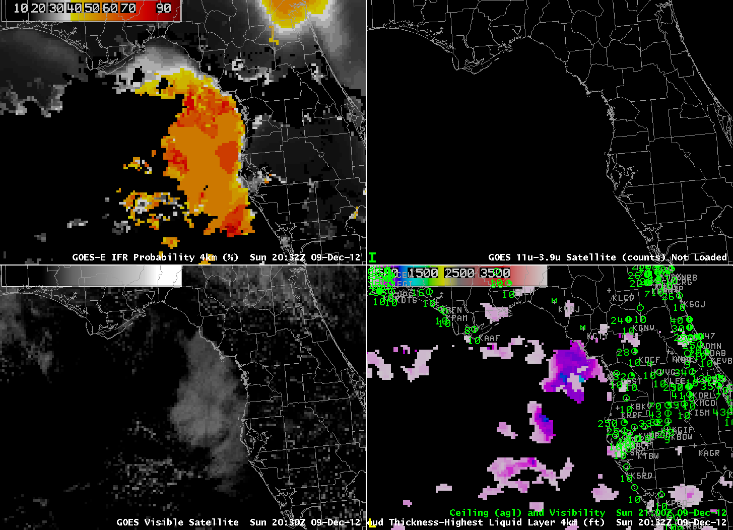
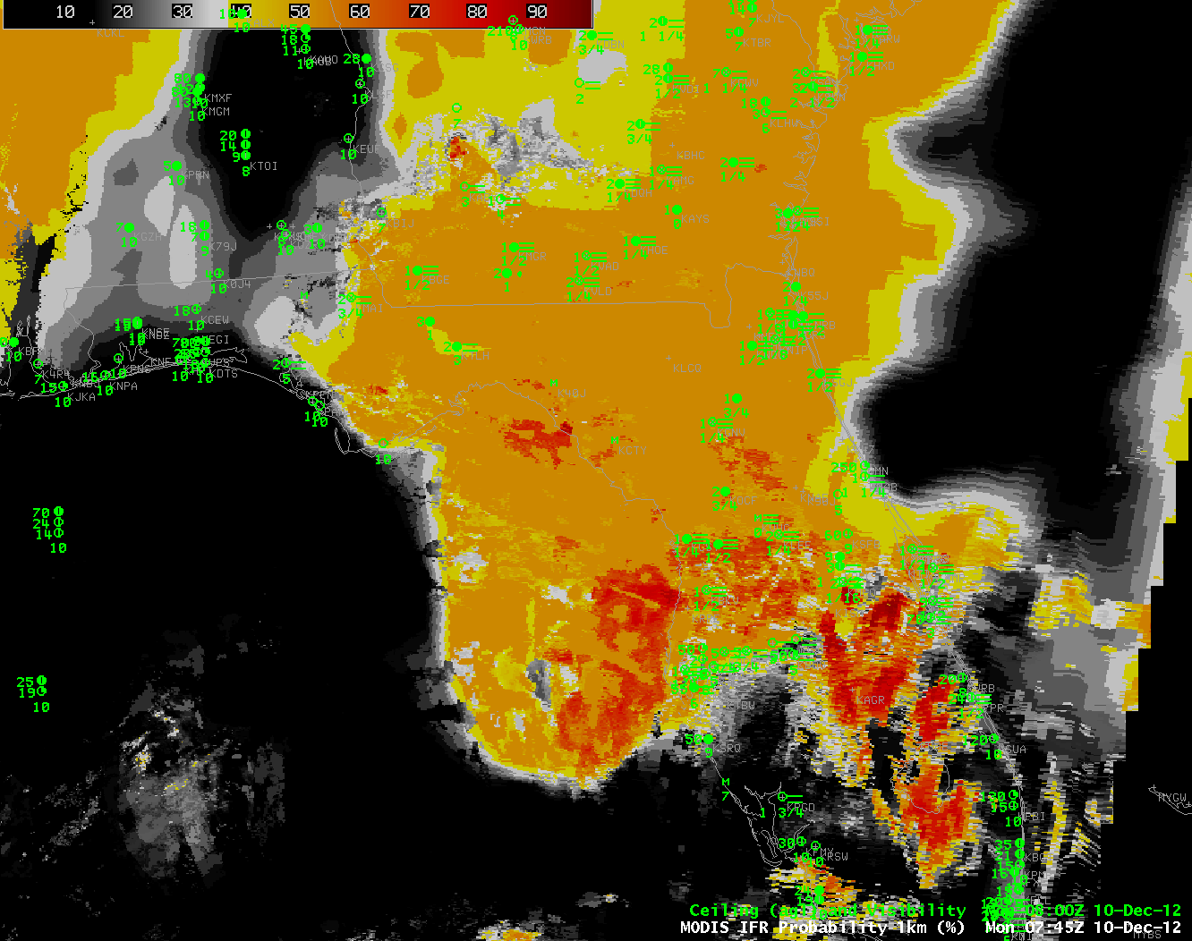
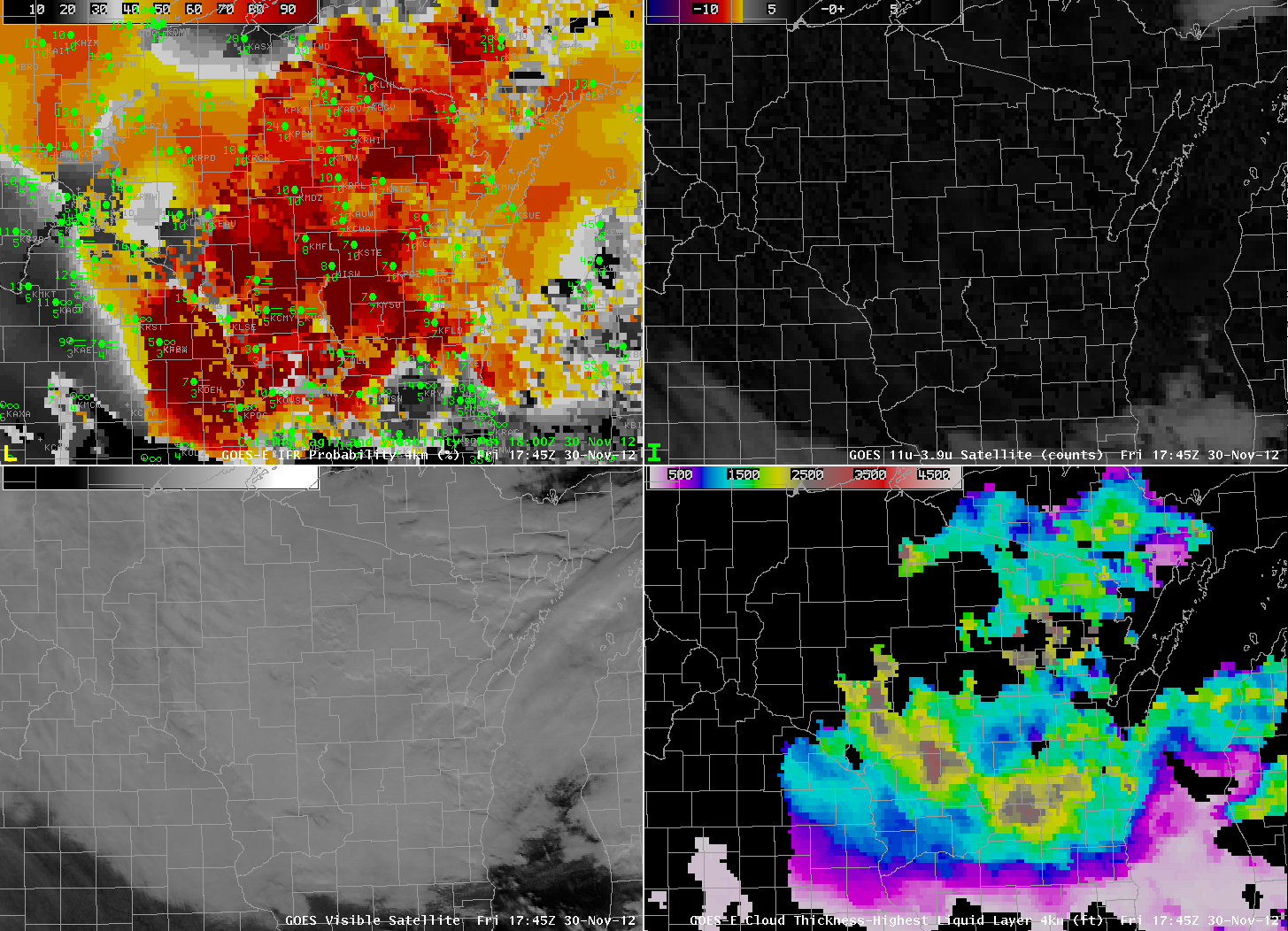
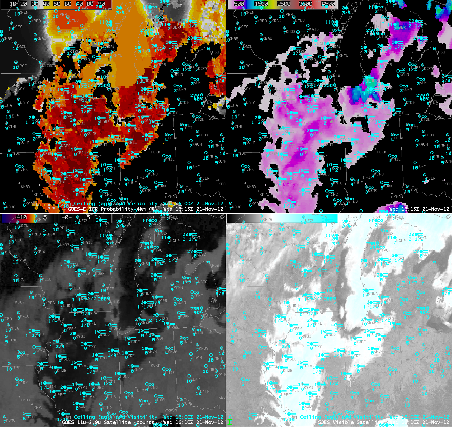
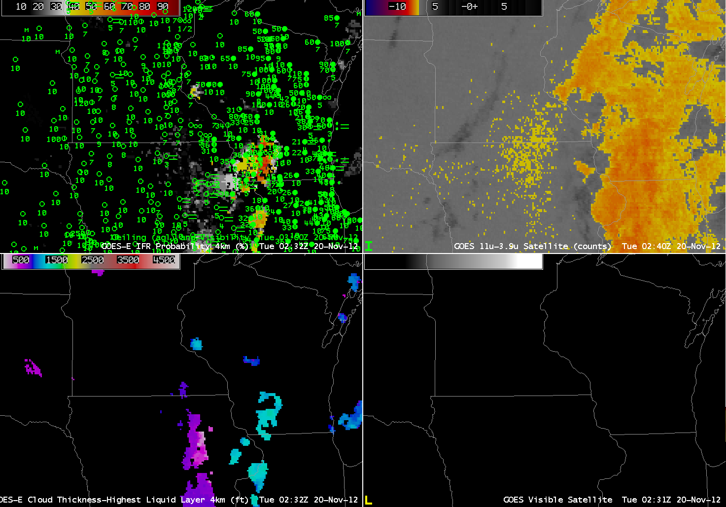
| GOES-R IFR Probabilities computed from GOES-East (upper left), GOES-East Traditional Brightness temperature difference, 10.7 µm – 3.9 µm (upper right), GOES-R Cloud Thickness (lower left), GOES-East Visible (0.63 µm ) imagery (lower right), from approximately 0230 UTC 20 Nov 2012. |
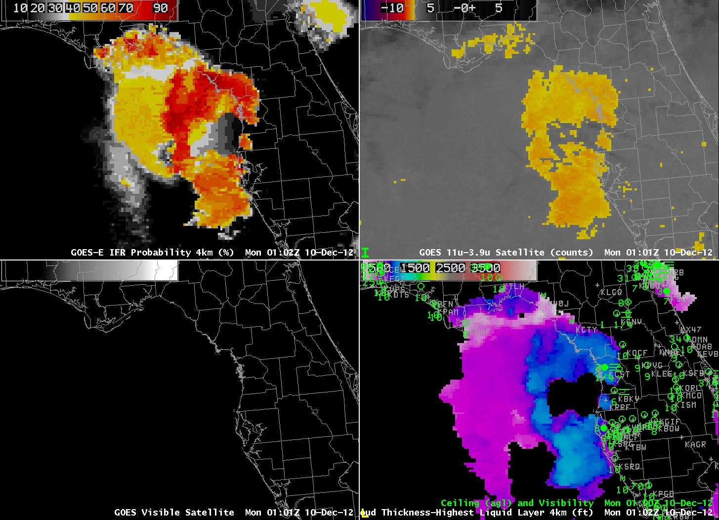
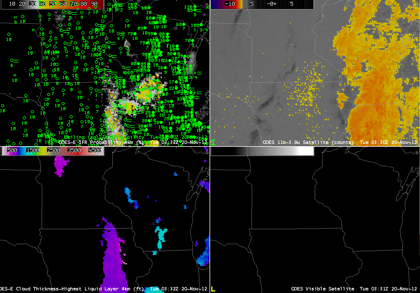
Dense fog developed over portions of the upper Mississippi Valley early in the morning on 20 November 2012. This event forced delayed openings for many eastern Iowa schools. How well did the GOES-R Fused Data products do for this event? The animation above shows the quick development of high IFR probabilities over Iowa; development over northwest Wisconsin, where IFR conditions were observed, was delayed. Why? The imagery above, from 0230 UTC, shows IFR probabilities increasing over eastern Iowa where near IFR conditions are already developing. At 0330 UTC, below, ceilings and visibilities continue to lower over eastern Iowa where IFR Probabilities increase. Note that the traditional brightness temperature difference field shows a strong signal over Wisconsin and Illinois — but IFR conditions there are not widespread, and IFR probabilities are except over southwest Wisconsin. The 0330 imagery also hints at higher clouds moving in from the west over southwest Minnesota and western Iowa/eastern Nebraska, where the darker regions in the brightness temperature difference product exists.
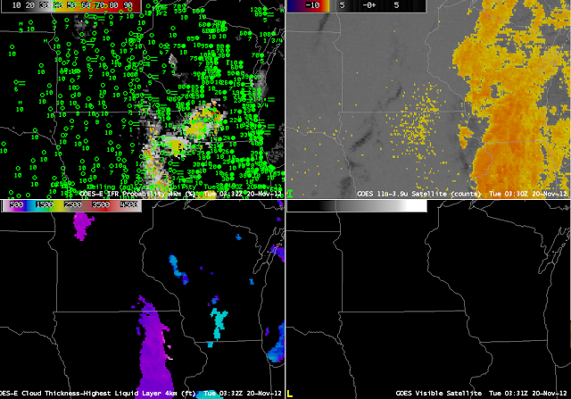 |
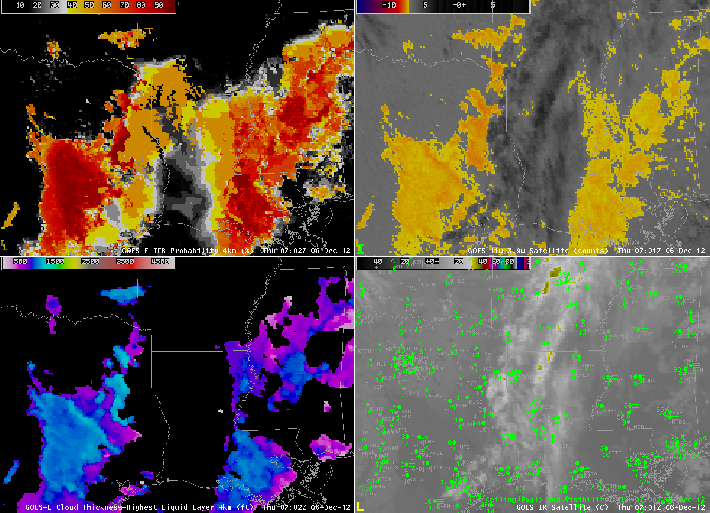
| GOES-R IFR Probabilities computed from GOES-East (upper left), GOES-East Traditional Brightness temperature difference, 10.7 µm – 3.9 µm (upper right), GOES-R Cloud Thickness (lower left), GOES-East Visible (0.63 µm ) imagery (lower right), from approximately 0330 UTC 20 Nov 2012. |
 |
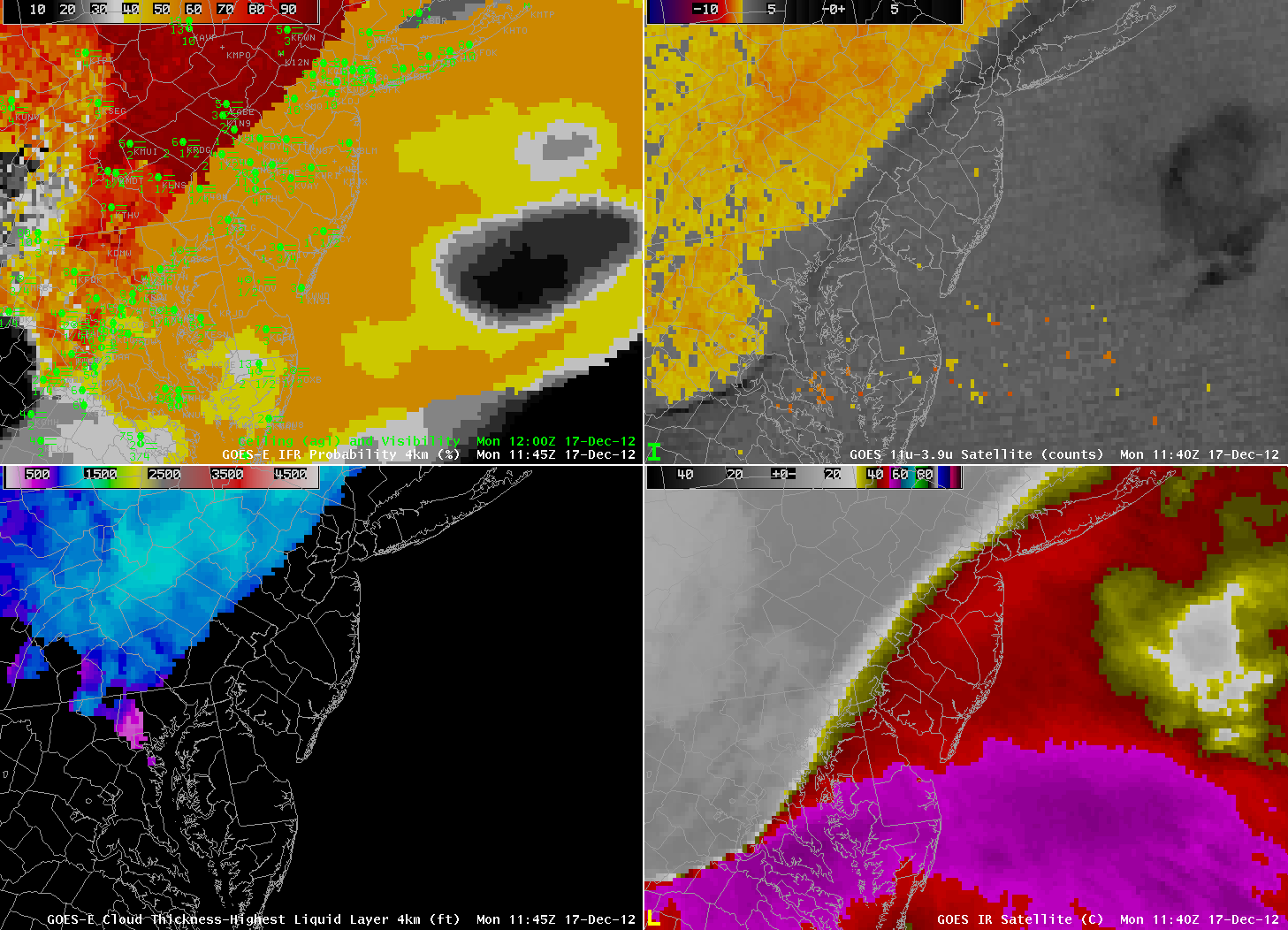
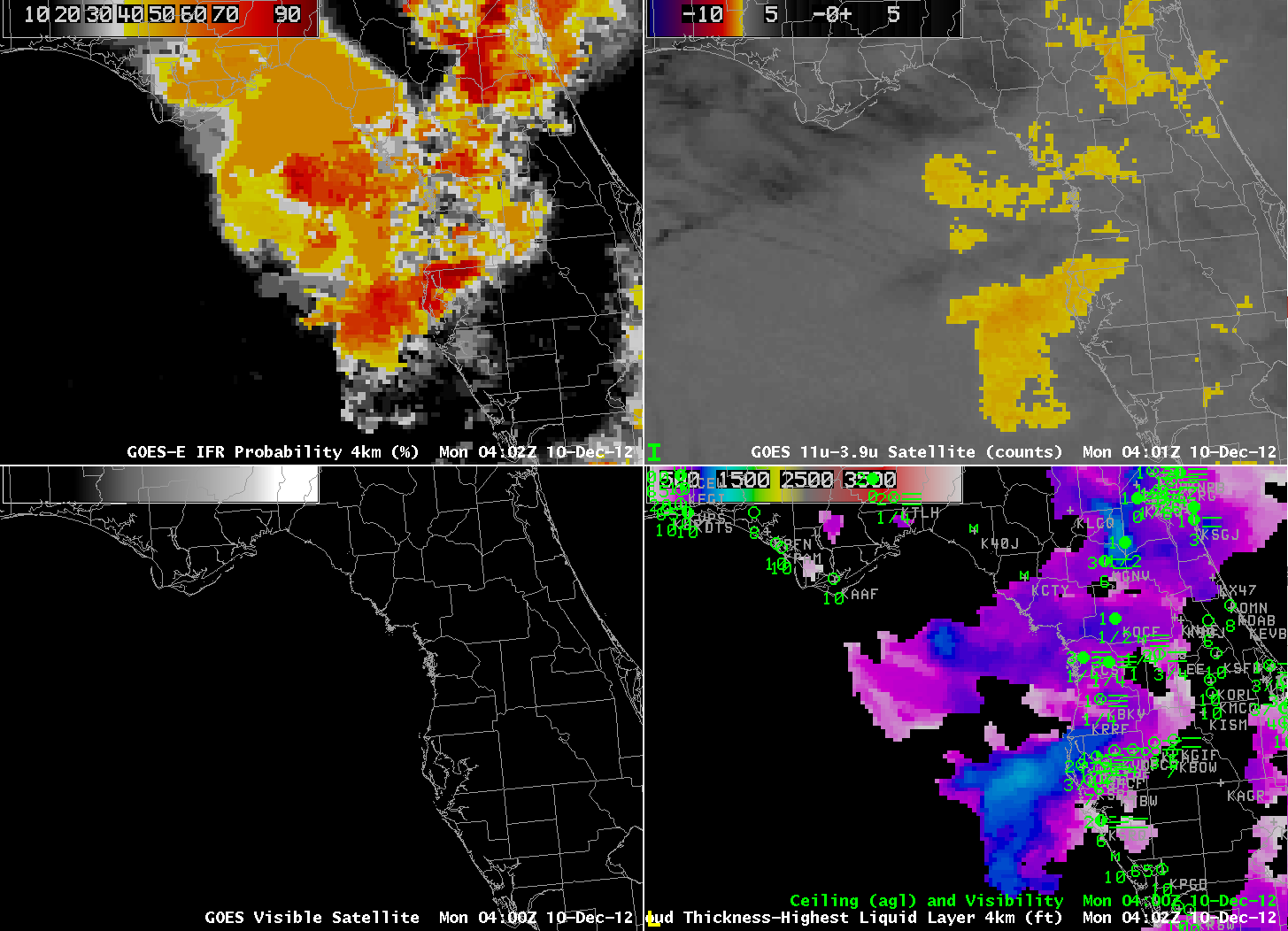
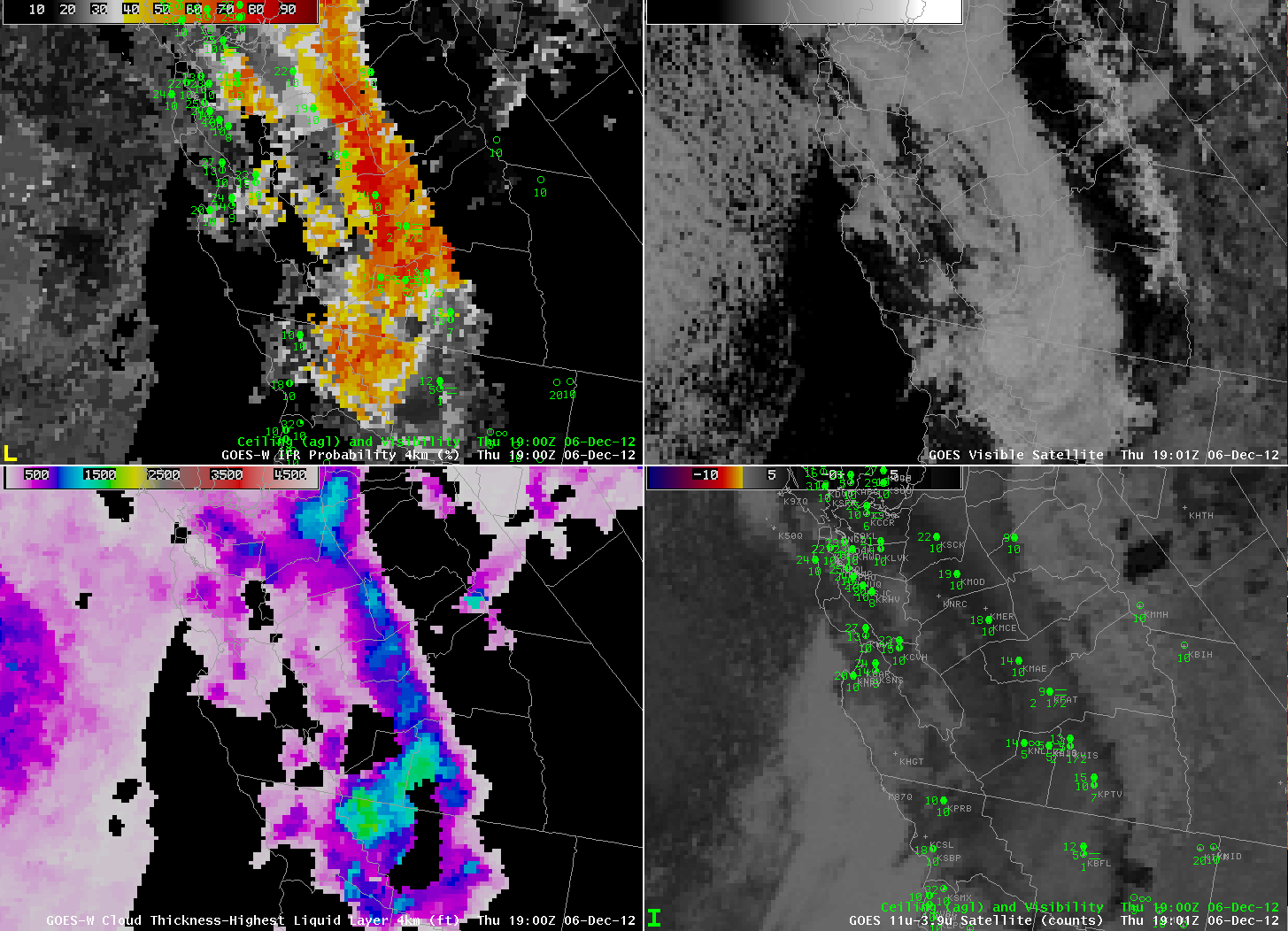
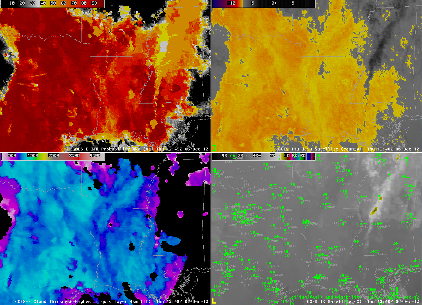
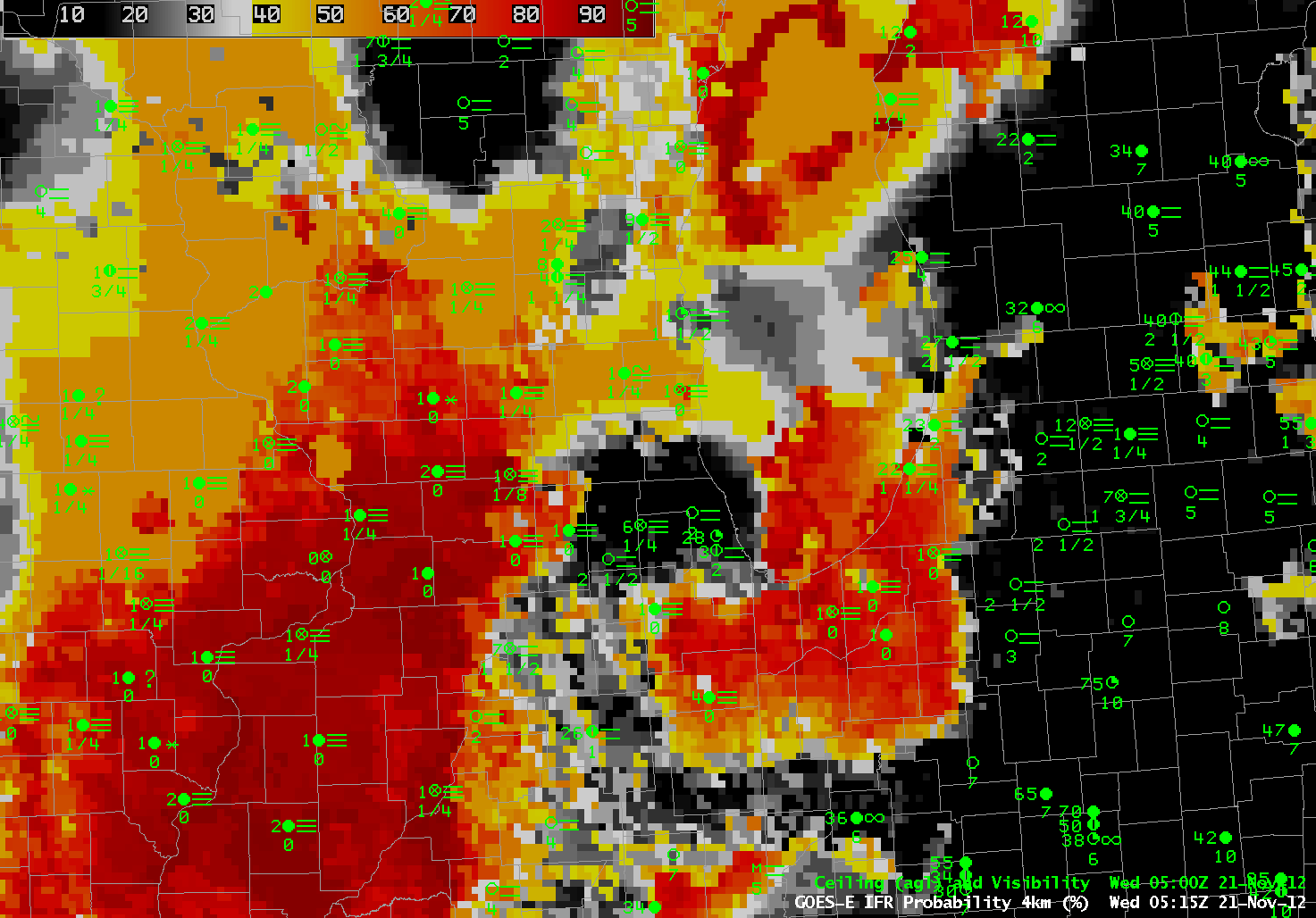
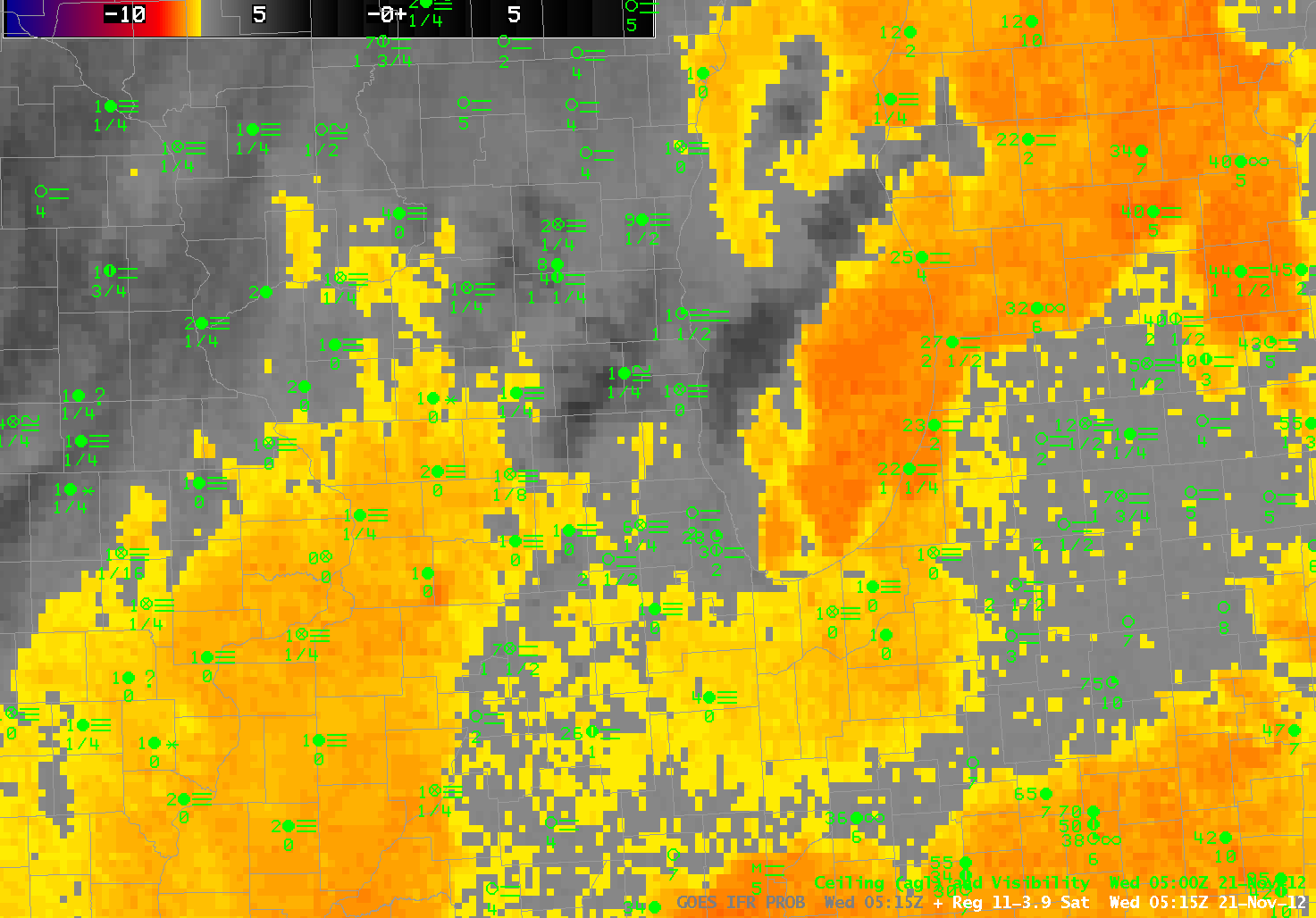
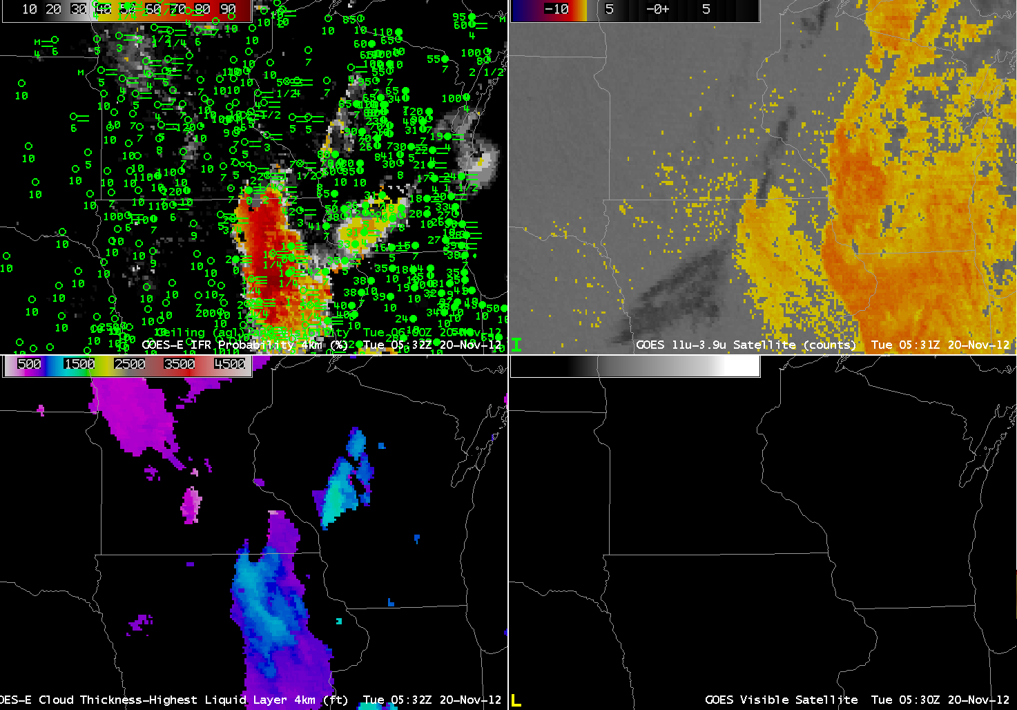
| GOES-R IFR Probabilities computed from GOES-East (upper left), GOES-East Traditional Brightness temperature difference, 10.7 µm – 3.9 µm (upper right), GOES-R Cloud Thickness (lower left), GOES-East Visible (0.63 µm ) imagery (lower right), from approximately 0530 UTC 20 Nov 2012. |
Two hours later, at 0530 UTC, IFR conditions are widespread over eastern Iowa where the traditional brightness temperature difference product has a signal, and where GOES-East-based GOES-R IFR Probabilities are very high. The Traditional brightness temperature difference signal from GOES-East continues to have a strong signal over central Wisconsin southward into Illinois where, except for southwest Wisconsin, IFR conditions are not common. Note the development of IFR conditions in northwest Wisconsin, in a region where IFR probabilities are low. In this region, satellite detection of low clouds is complicated by higher clouds (indicated by the dark region in the brightness temperature difference product). In addition, low-level relative humidity fields at this time in the Rapid Refresh model are lower than they are over Iowa (see the animation of fields used to compute IFR probabilities at the bottom of this post).
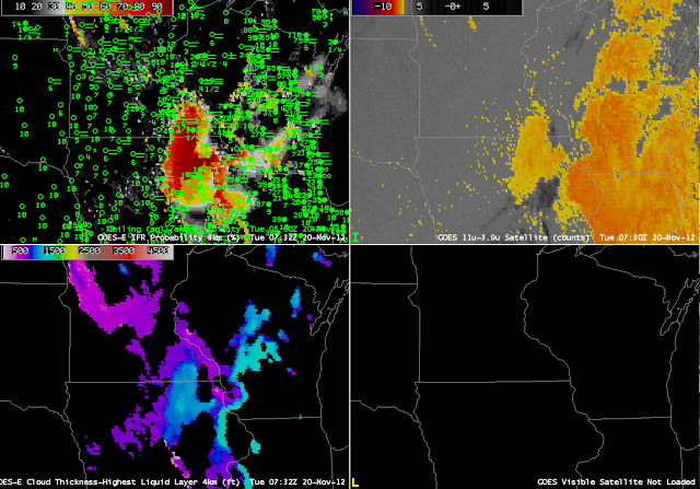 |
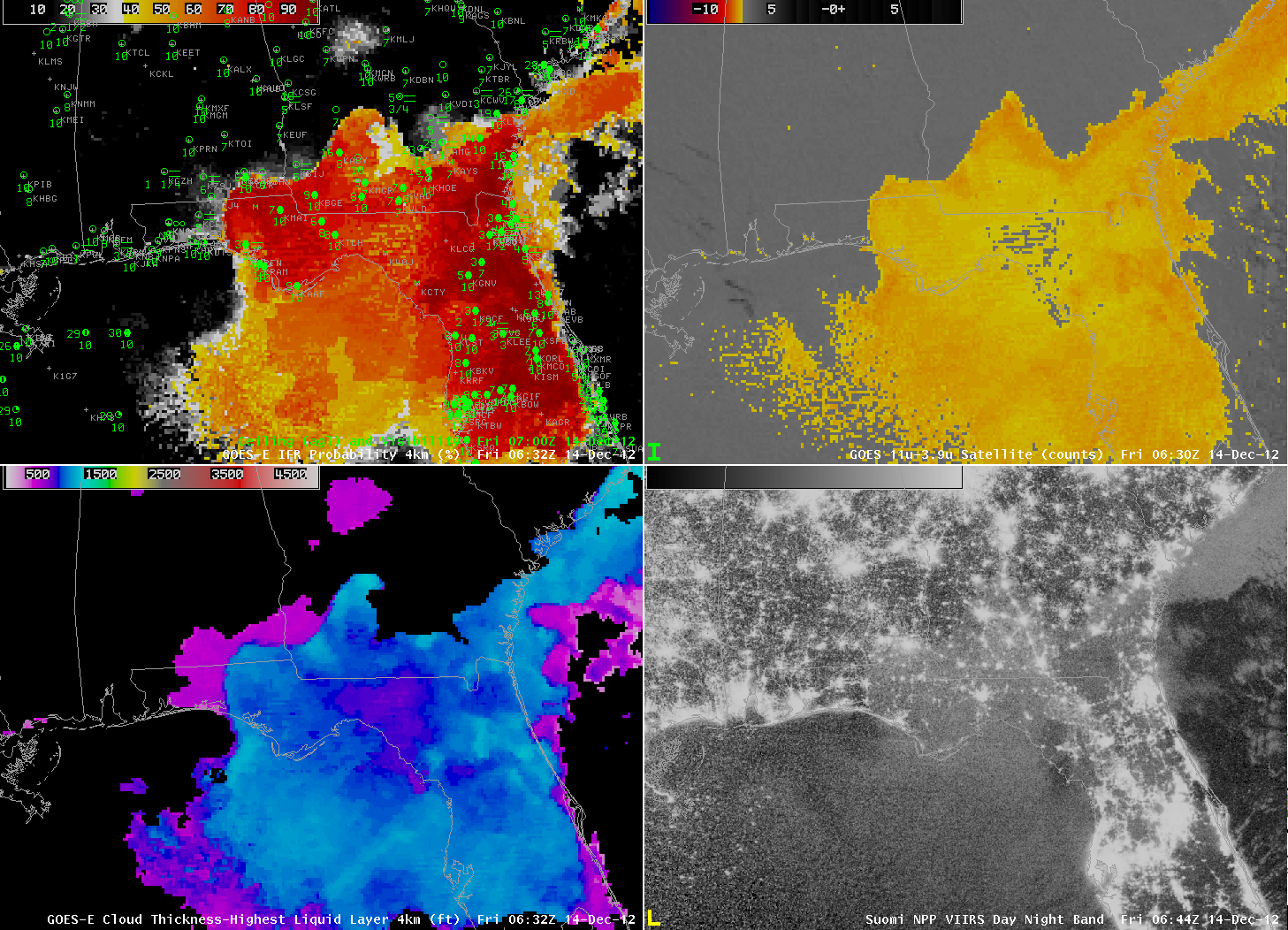
| GOES-R IFR Probabilities computed from GOES-East (upper left), GOES-East Traditional Brightness temperature difference, 10.7 µm – 3.9 µm (upper right), GOES-R Cloud Thickness (lower left), GOES-East Visible (0.63 µm ) imagery (lower right), from approximately 0730 UTC 20 Nov 2012. |
At 0730 UTC, above, mid-level clouds over eastern Iowa are having an effect on IFR probabilities there. Because satellite predictors cannot give a strong indication of fog/low stratus when mid-level (or higher) clouds are present, IFR probabilities will decrease. This is happening over portions of eastern Iowa where IFR conditions persist. Probabilities fall, and the field acquires a much smoother look; in addition, Cloud thickness is not computed. These occurrences all are a consequence of the presence of higher clouds, as depicted by the darker grey enhancement in the traditional brightness temperature difference field. Note that IFR probabilities continue to be fairly low over northwest Wisconsin where IFR or near-IFR conditions are present.
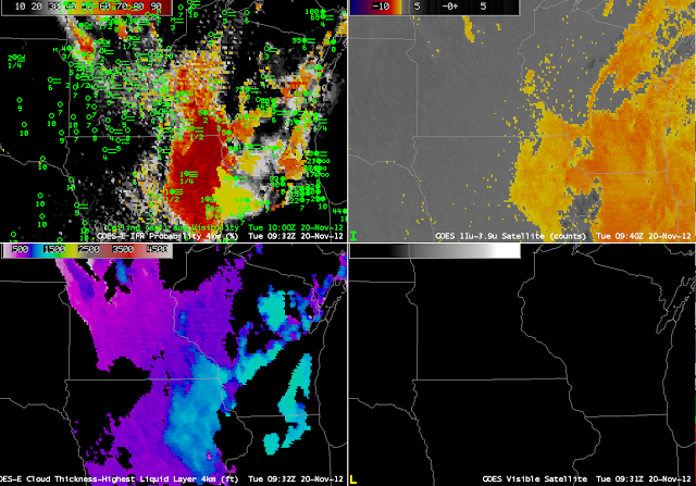 |
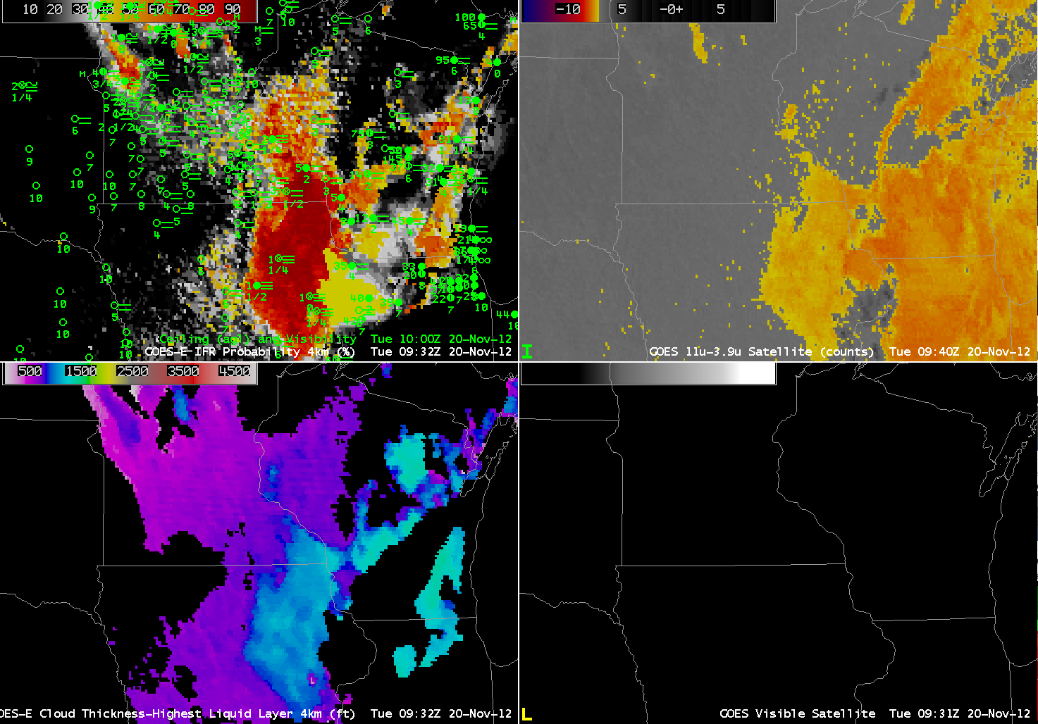
| GOES-R IFR Probabilities computed from GOES-East (upper left), GOES-East Traditional Brightness temperature difference, 10.7 µm – 3.9 µm (upper right), GOES-R Cloud Thickness (lower left), GOES-East Visible (0.63 µm ) imagery (lower right), from approximately 0930 UTC 20 Nov 2012. |
By 0930 UTC, IFR probabilities finally do increase over northwest Wisconsin where IFR or near-IFR conditions are present (similarly, they increase over eastern Wisconsin near Lake Michigan). Both the satellite signal and the Rapid Refresh signal have started to suggest low clouds near the surface, as observed. An animation of fields important to the computation of IFR probabilities is below. Note how the near-surface relative humidity saturates first over eastern Iowa; that saturation is slow to spread northward into northwest Wisconsin.
 |
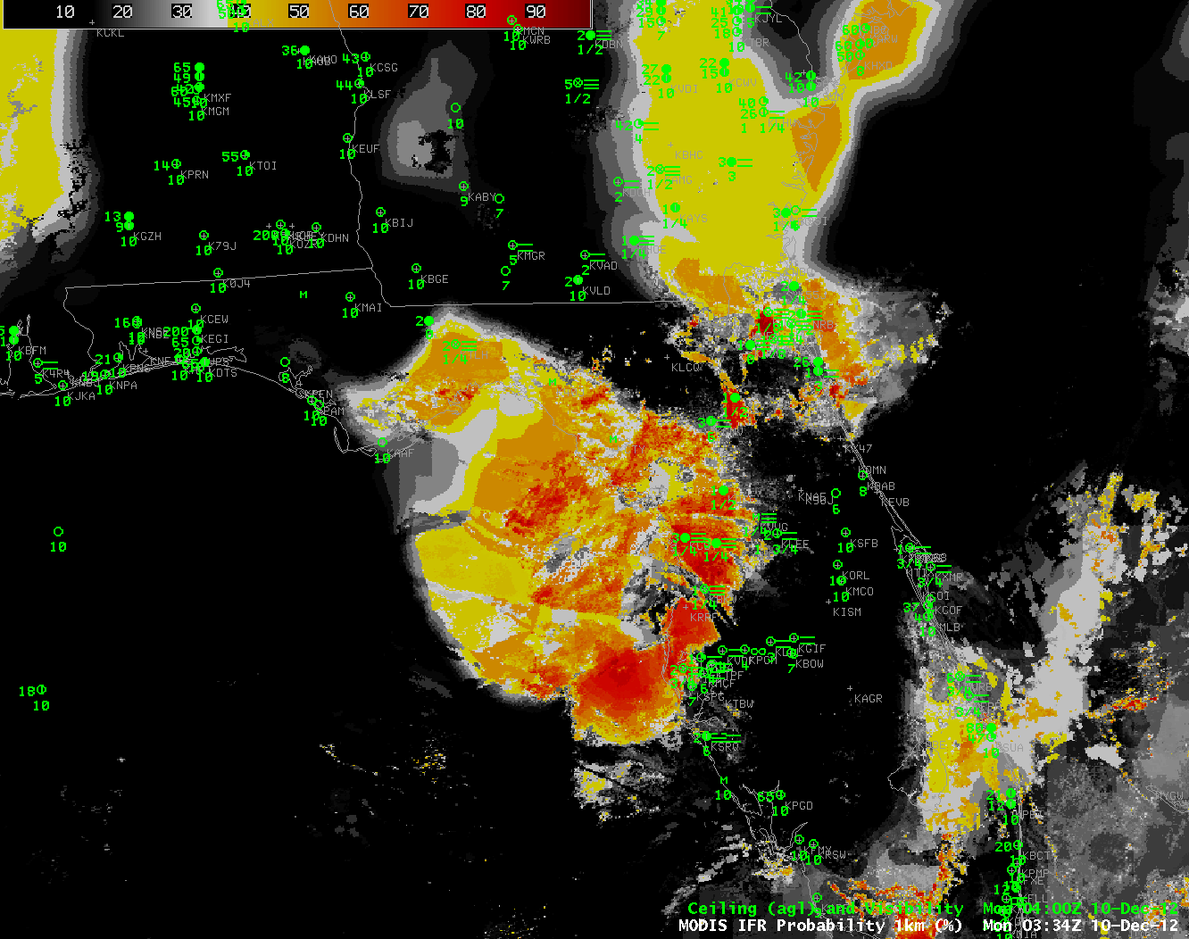
| Heritage Fog Algorithm (10.7 µm – 3.9 µm ) from GOES-East (upper left, white = fog/low stratus), GOES-R Cloud Type (upper right), GOES-East 10.7 µm imagery (lower left), Peak Rapid Refresh Model Relative Humidity below 500 m (lower right), hourly from 0432 UTC through 0932 UTC, 20 November 2012. Data from this site. |
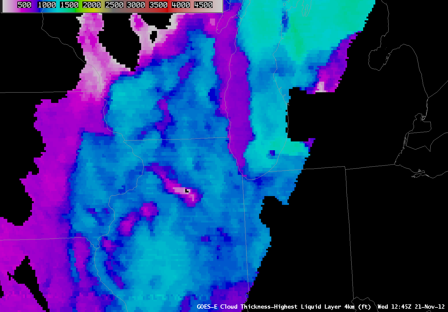
The last pre-twilight Cloud Thickness product can be used to guess the dissipation of radiation fog. Those data are shown below. Cloud thickness over eastern Iowa and southwest Wisconsin peaks around 1200 feet. This graph suggests, then, a dissipation time about 5 hours after sunrise.
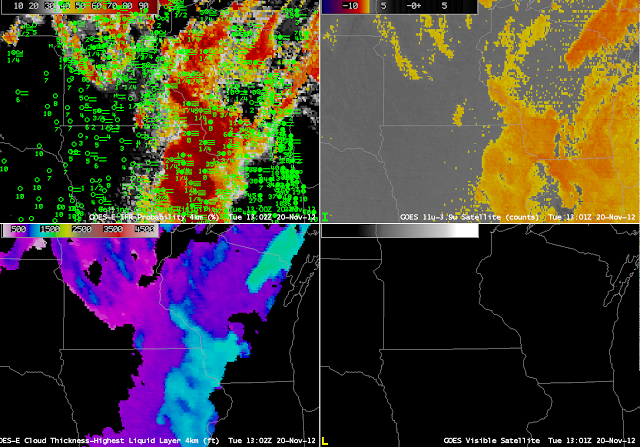 |
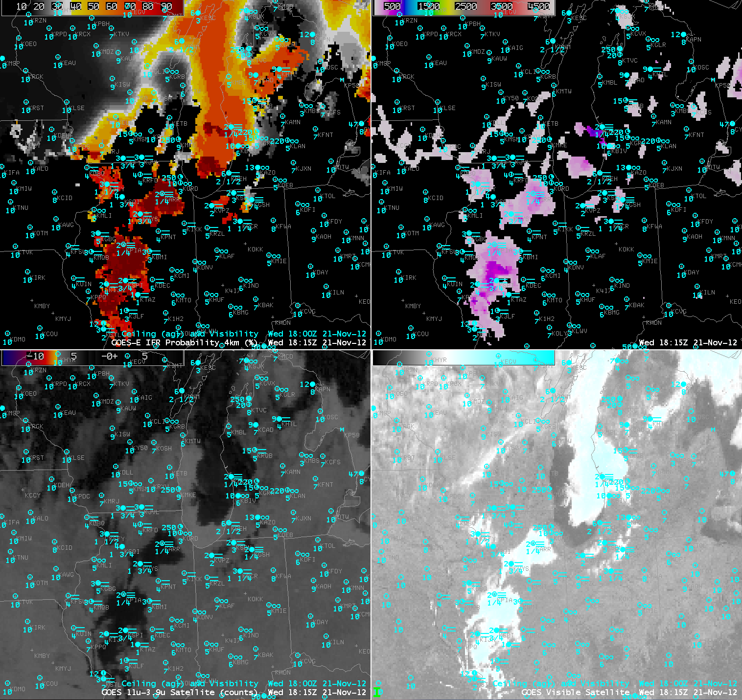
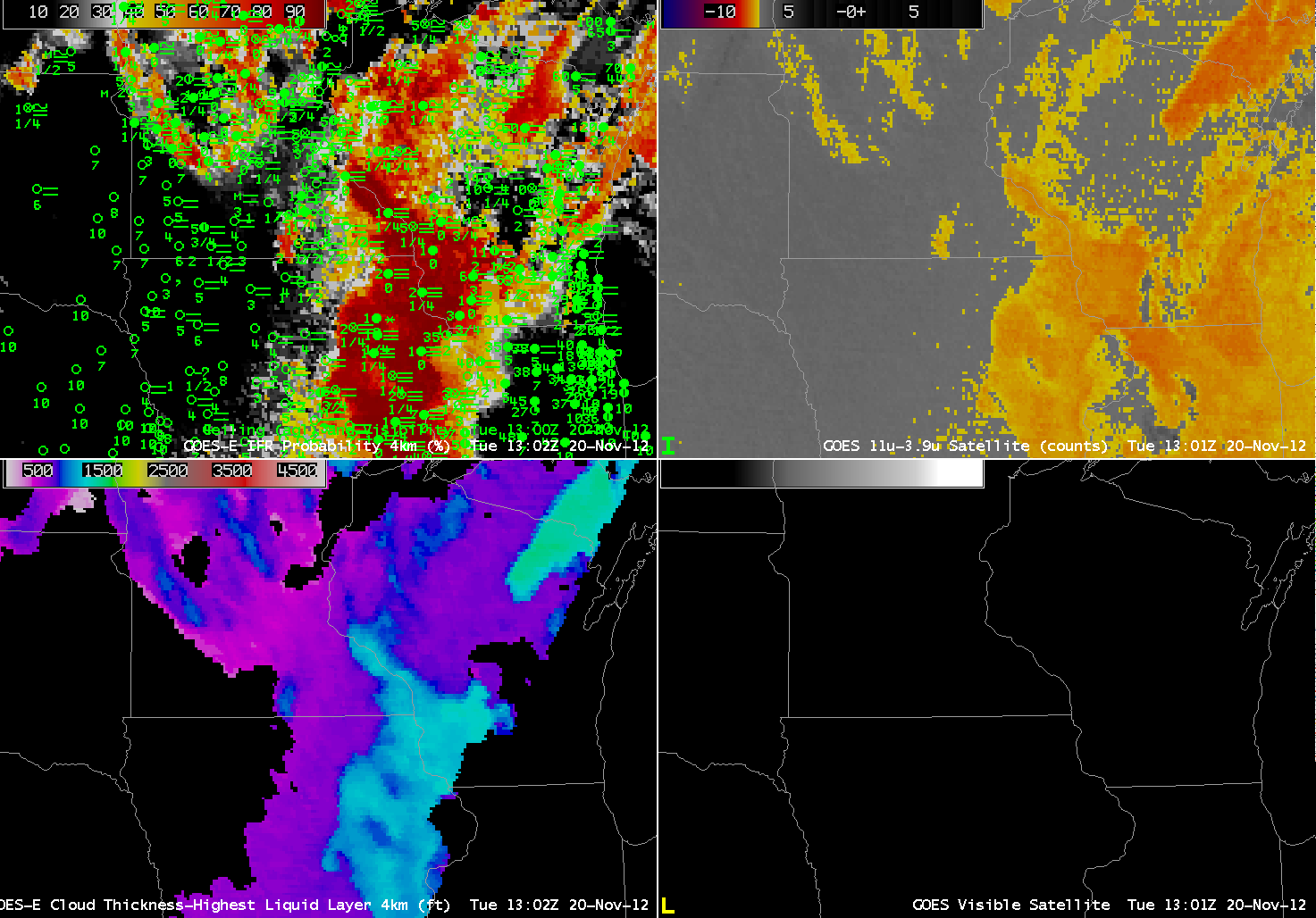
| GOES-R IFR Probabilities computed from GOES-East (upper left), GOES-East Traditional Brightness temperature difference, 10.7 µm – 3.9 µm (upper right), GOES-R Cloud Thickness (lower left), GOES-East Visible (0.63 µm ) imagery (lower right), from approximately 1300 UTC 20 Nov 2012. |
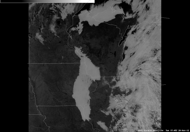 |
| GOES-East Visible Imagery, 1745 UTC |
Note how well the low clouds over eastern Iowa at 1745 UTC align with the cloud thickness field at 1300 UTC!
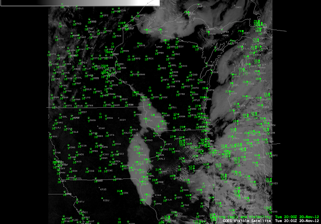 |
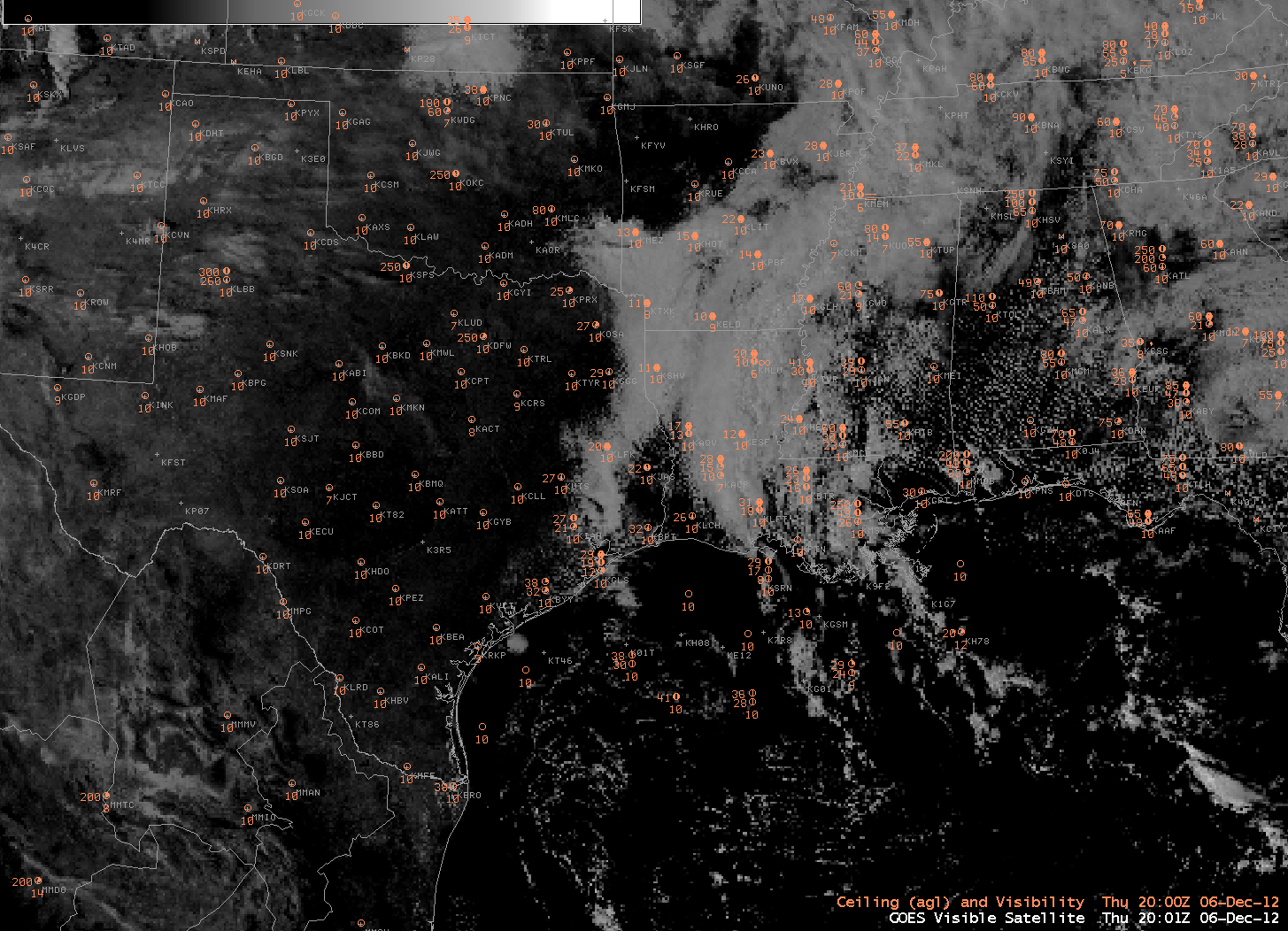
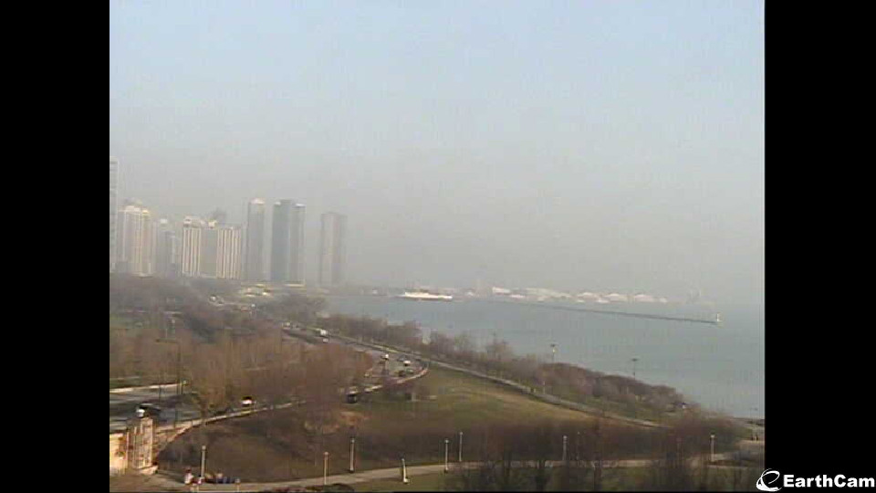
| GOES-East visible imagery and station ceilings/visibilities, 2002 UTC |
(Update: The low sun angle of mid- to late-November is making it difficult for the fog to burn off. As of 2000 UTC, stratus persists)


