Category Archives: Cloud Thickness

GOES-R vs. Heritage GOES Fog Products in Arkansas

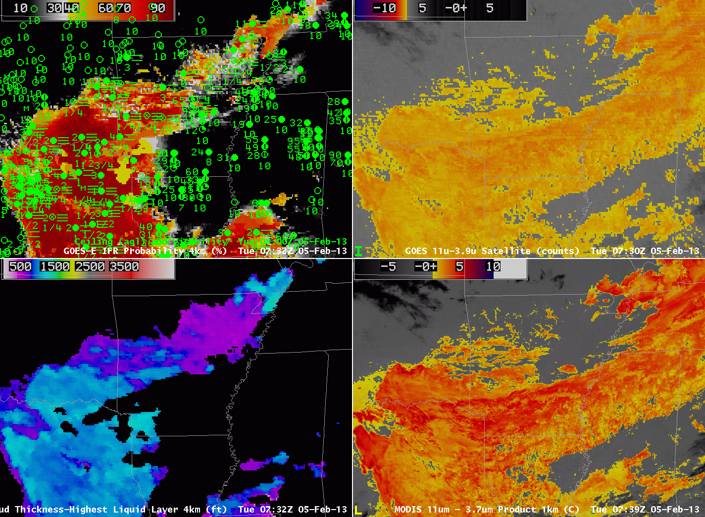
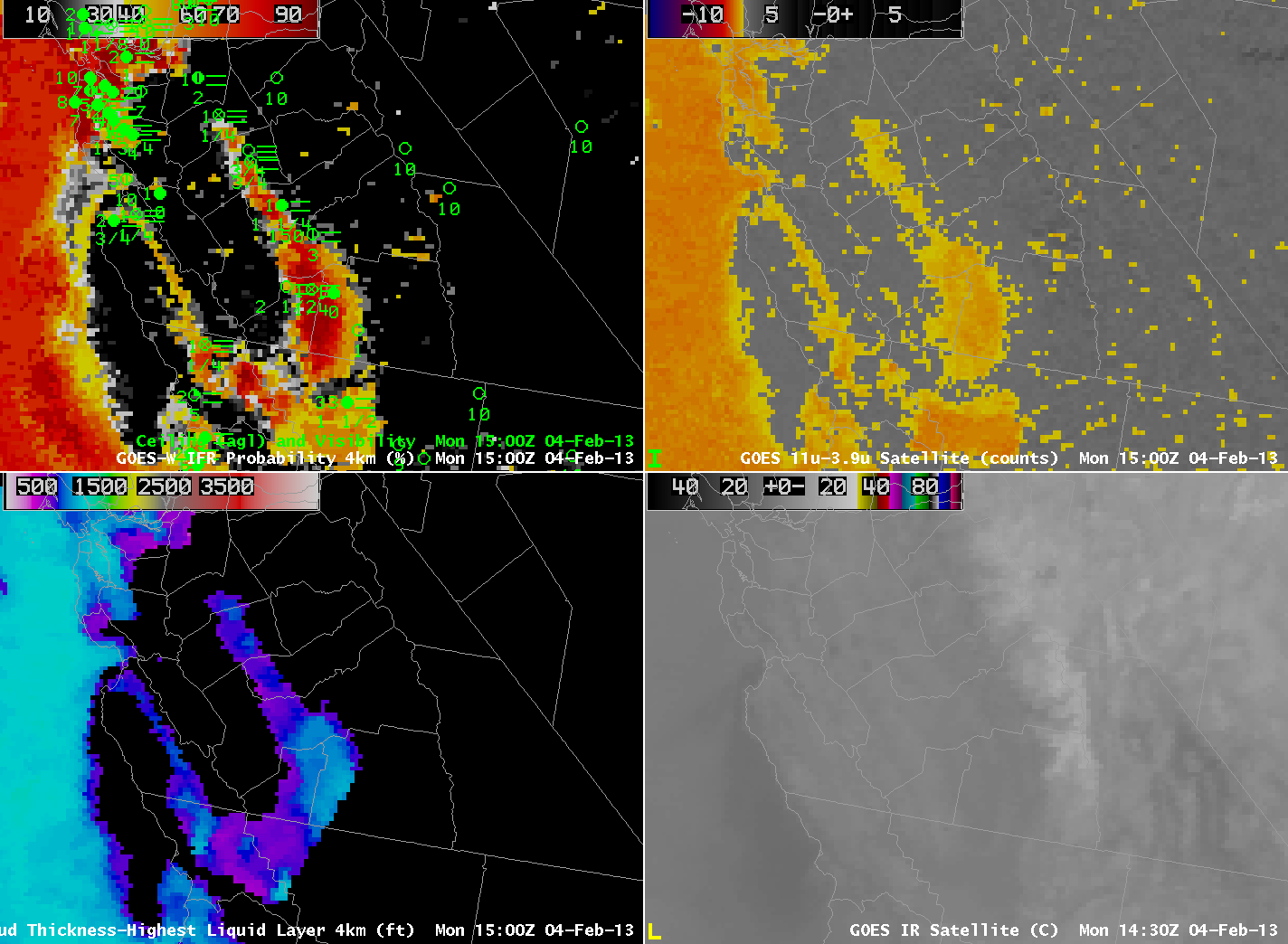
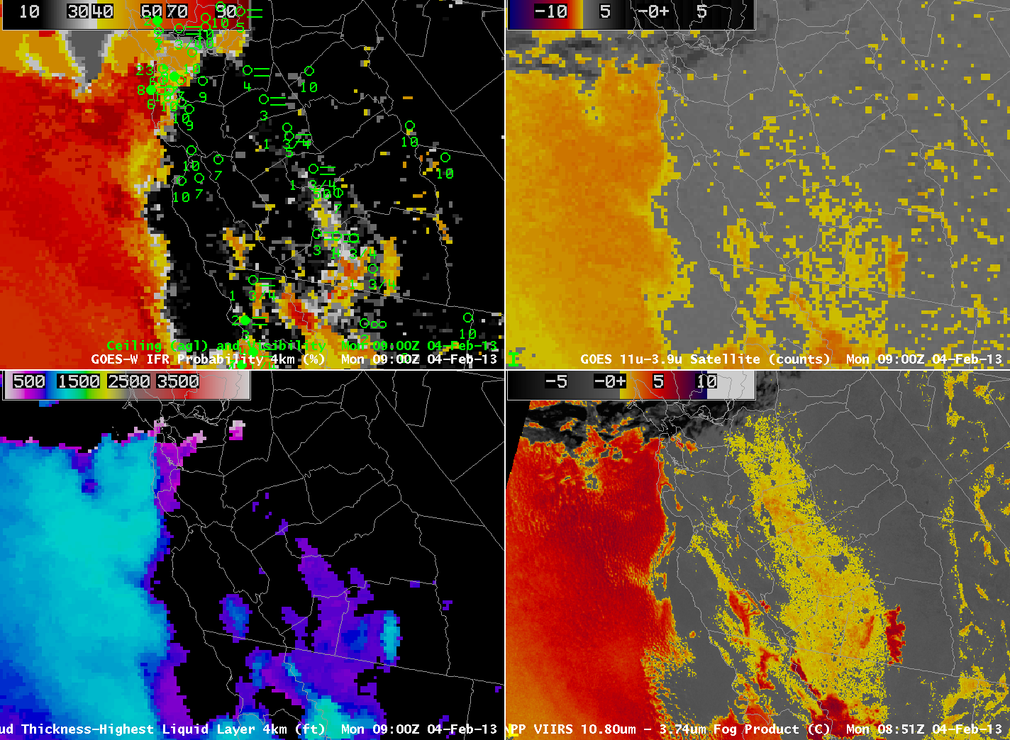
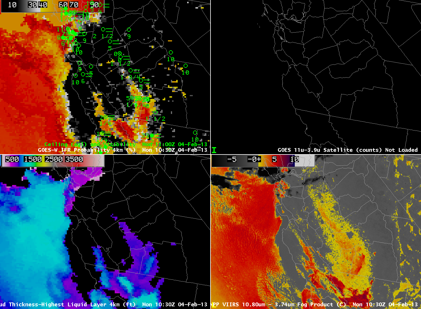
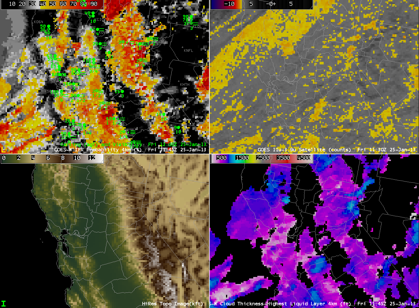
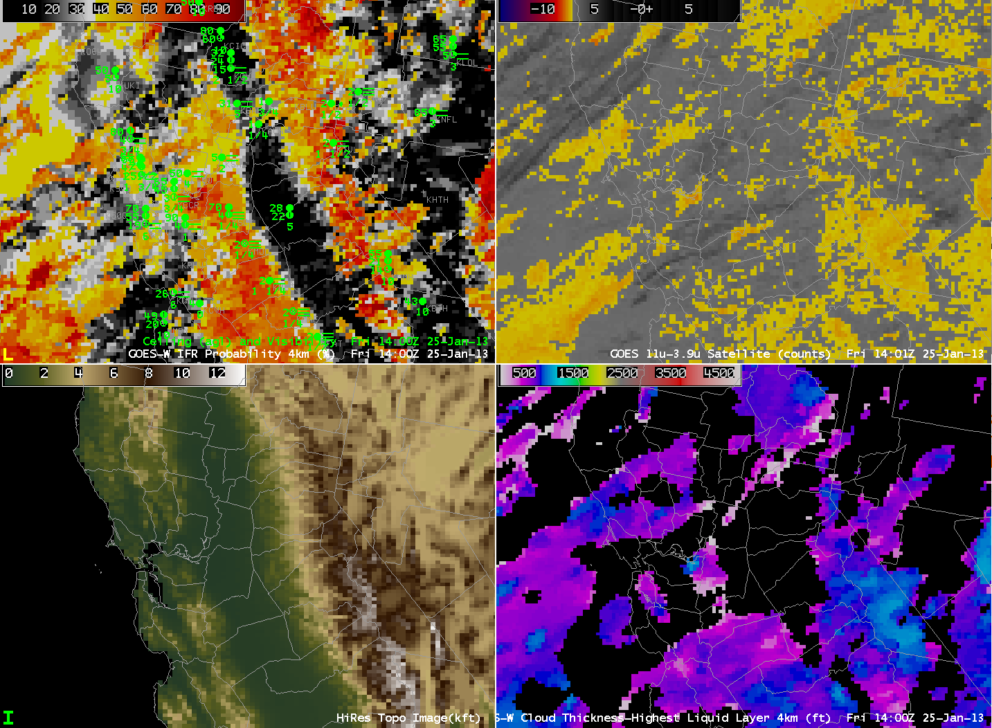
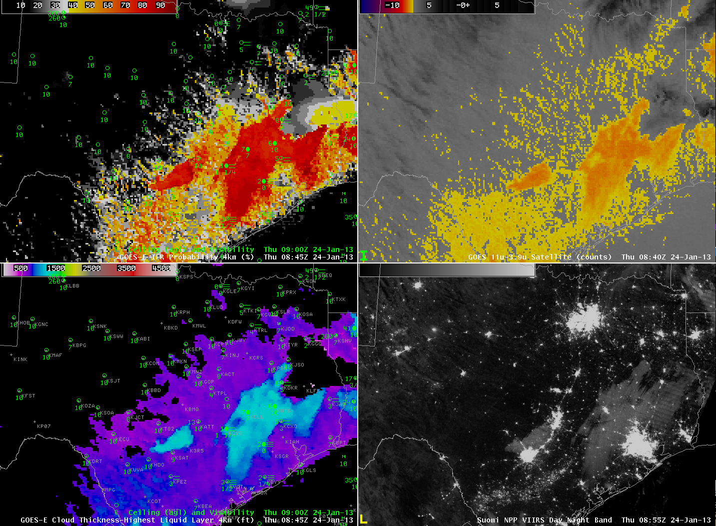
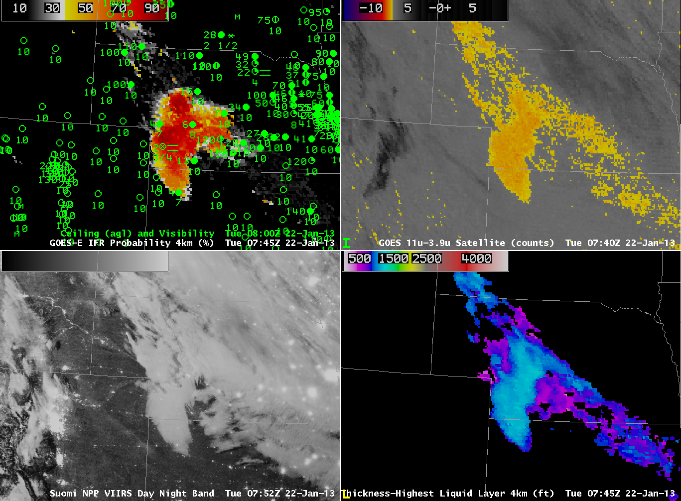
GOES-R IFR Probabilities, from GOES-East (0732 UTC) and 0800 UTC Surface observations of visibility and ceilings (Upper Left), GOES-E Brightness Temperature Difference (10.8 µm – 3.9 µm) (Upper Right), GOES-R Cloud Thickness (Lower Left), MODIS-based Brightness Temperature Difference (11µm – 3.74 µm) GOES-R IFR Probabilities computed using MODIS data (Lower Left, 0739 UTC)

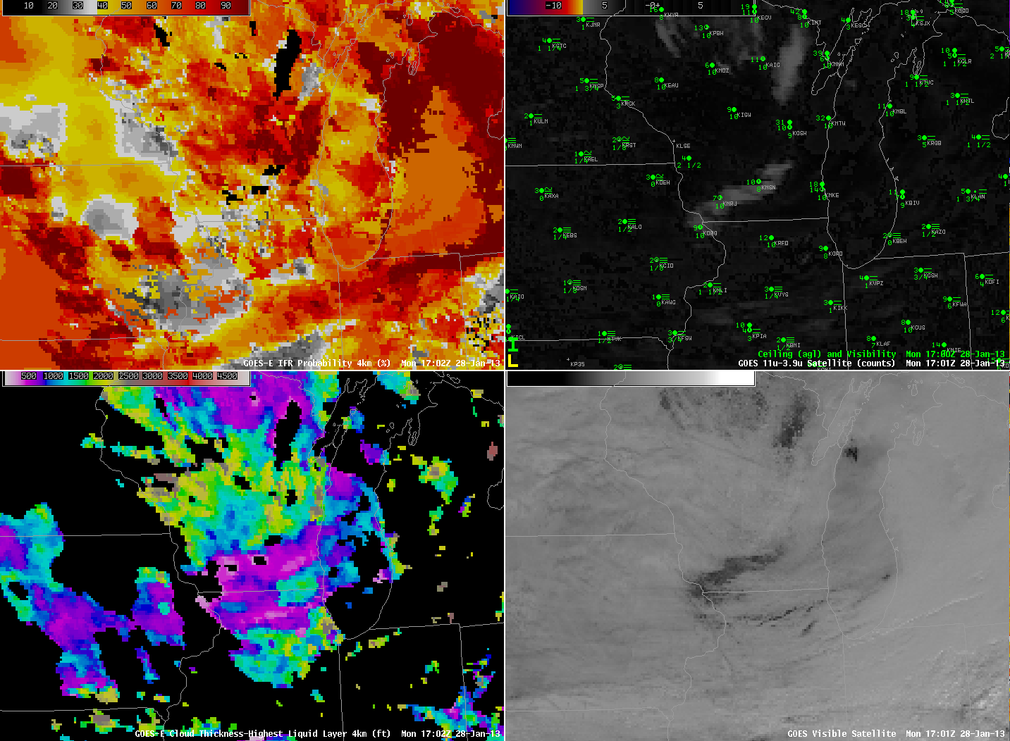
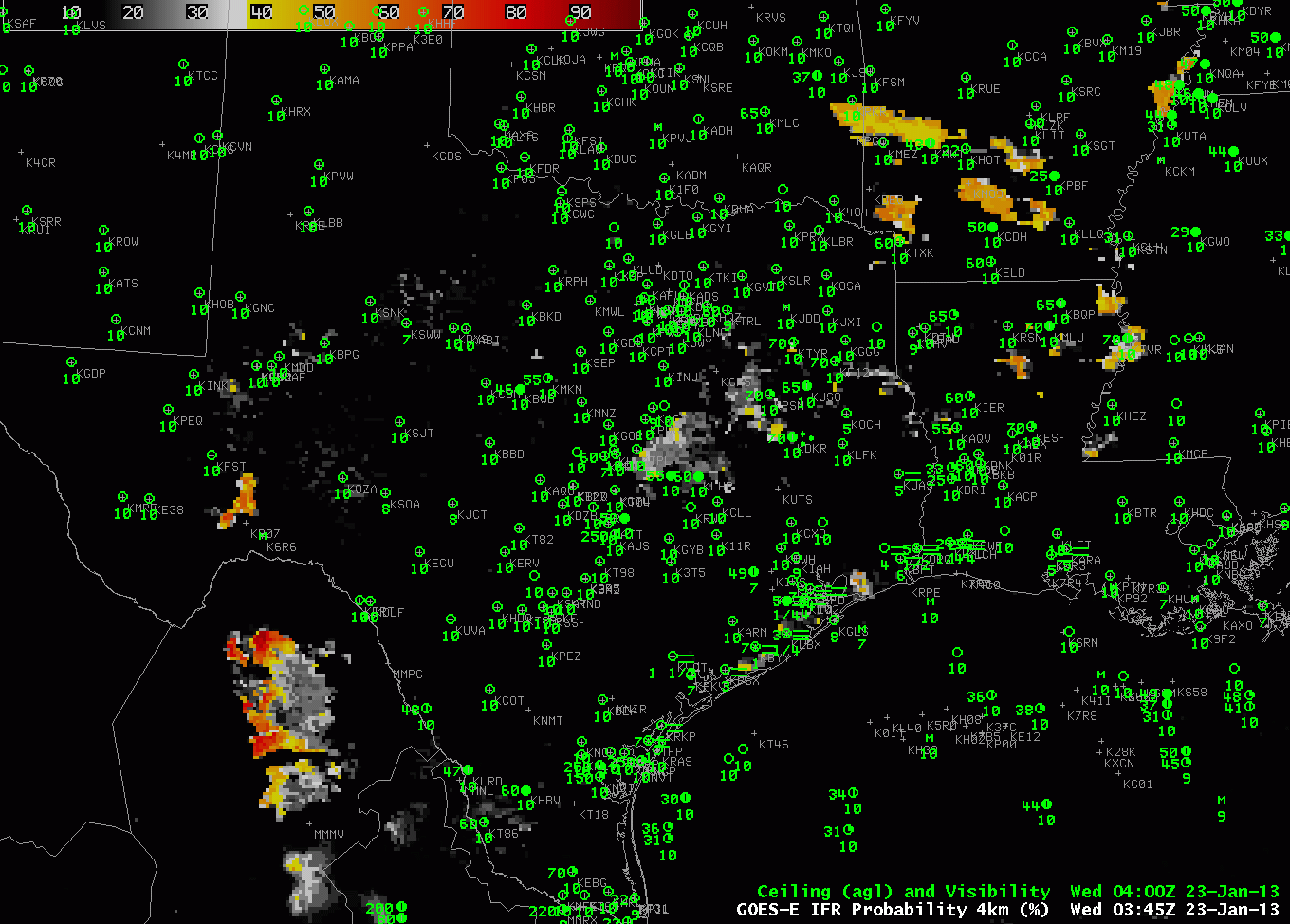
IFR conditions developed over Arkansas and surrounding states overnight from 4 into 5 February.  Compare the brightness temperature difference (the traditional fog-detection product) over southeast Arkansas (where IFR conditions are not occurring) and over southwest Arkansas (where IFR conditions are present).  Although the satellite signal is very similar over the region, surface observations are very different.  The GOES-R algorithm distinguishes between the region with IFR conditions (east Texas, western Arkansas, northwest Louisiana) and the region without IFR conditions (southeast Arkansas, northeast Louisiana).

On the flip side, in regions over northeast Arkansas, where the brightness temperature difference product is not showing low clouds, IFR conditions are present, and the GOES-R IFR probability is elevated.

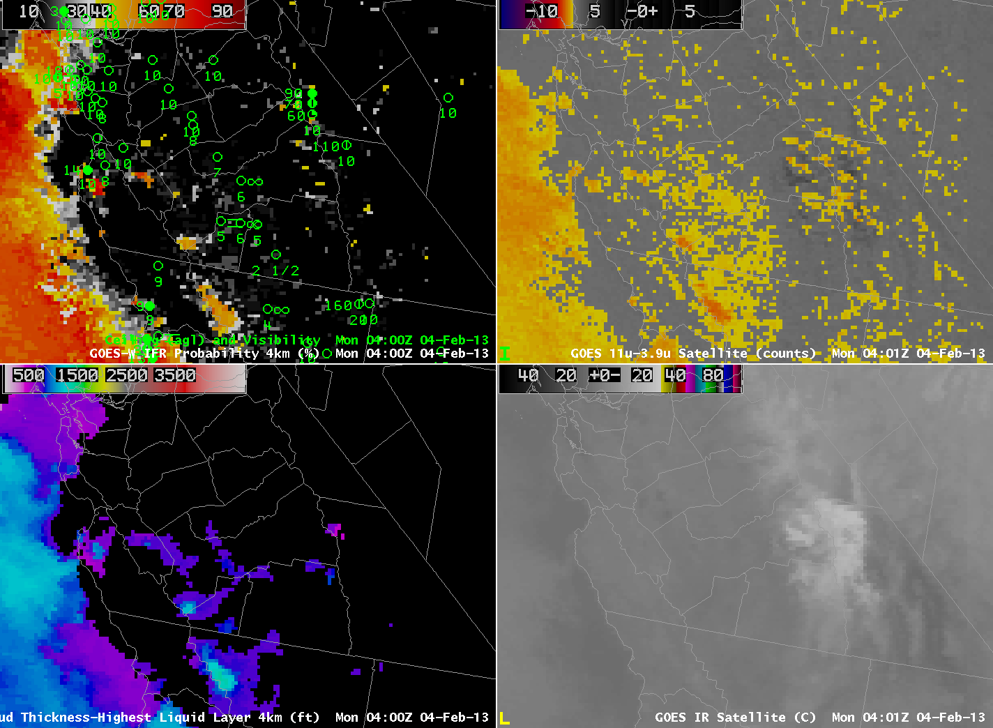
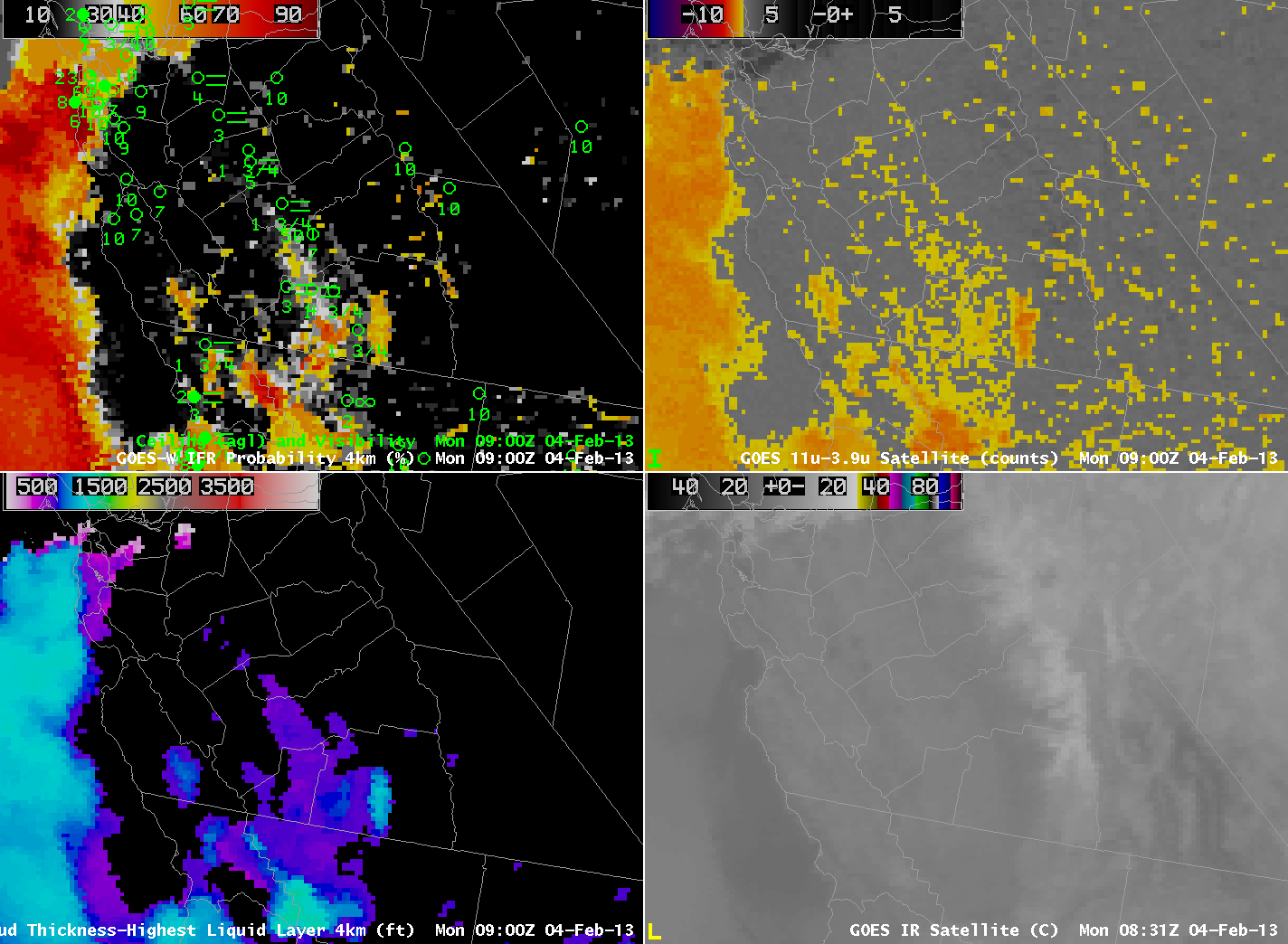
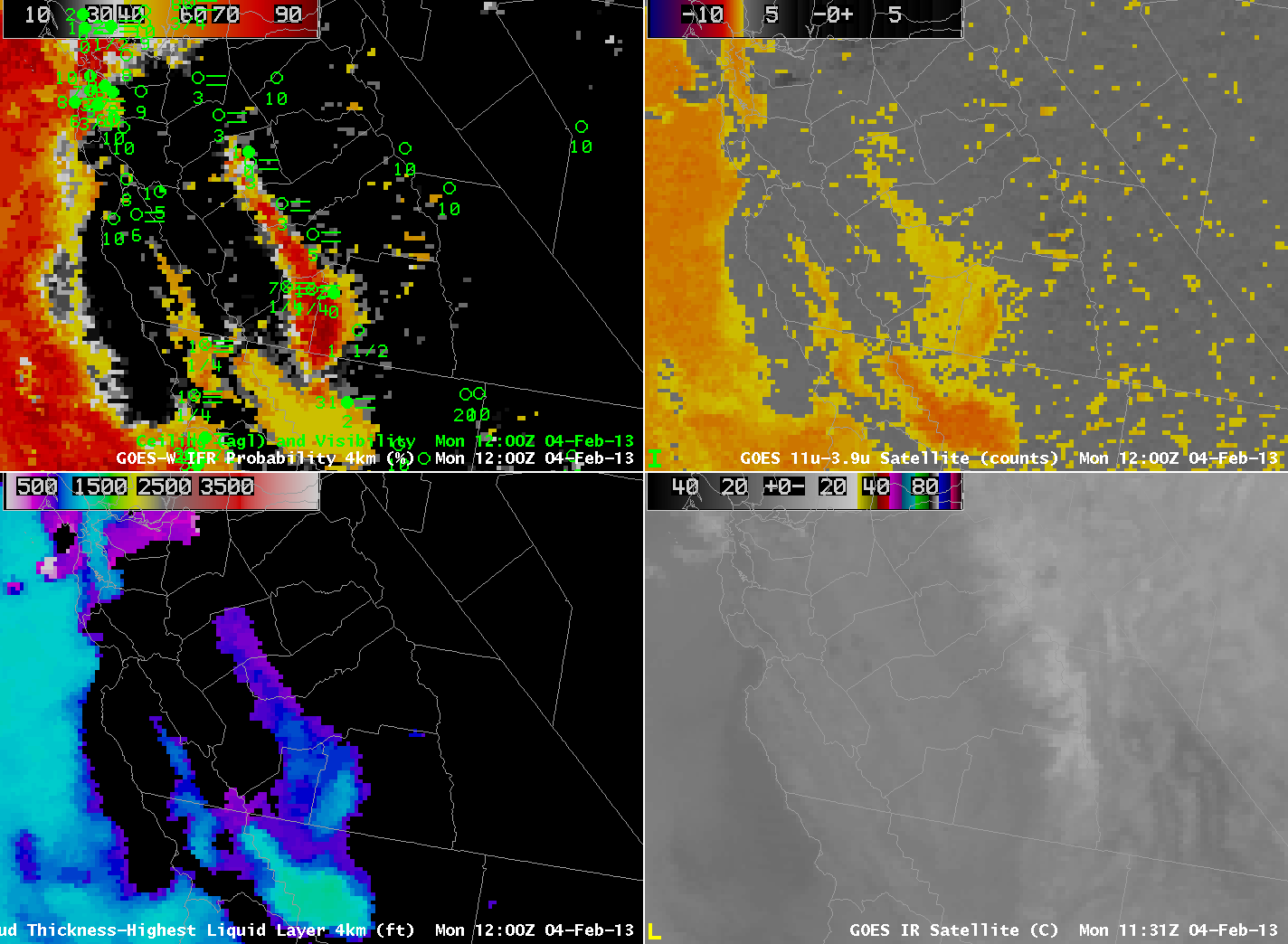
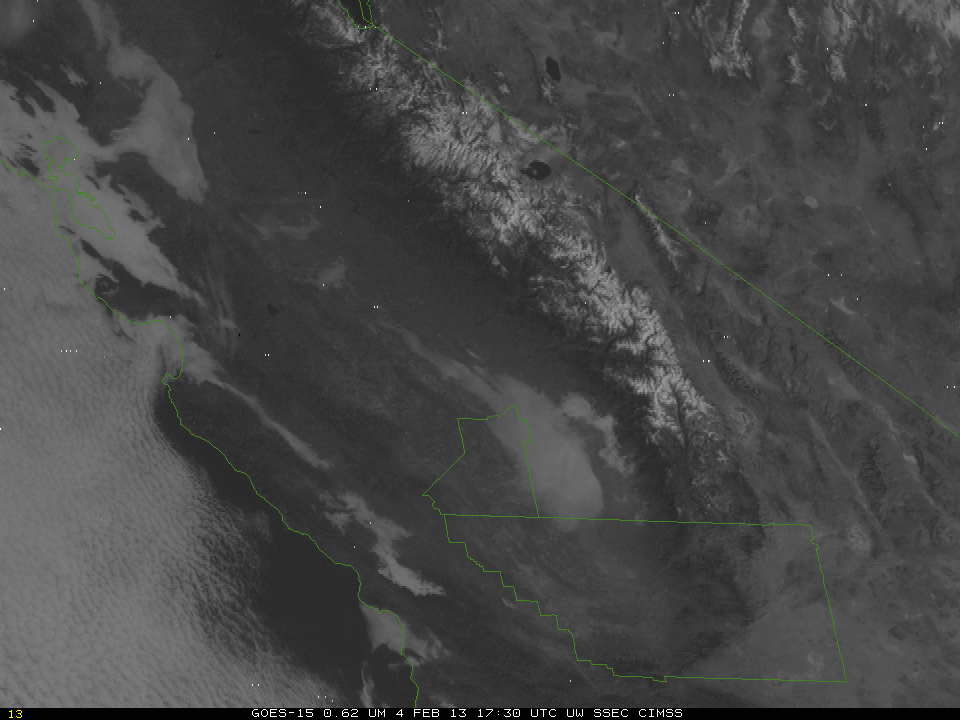
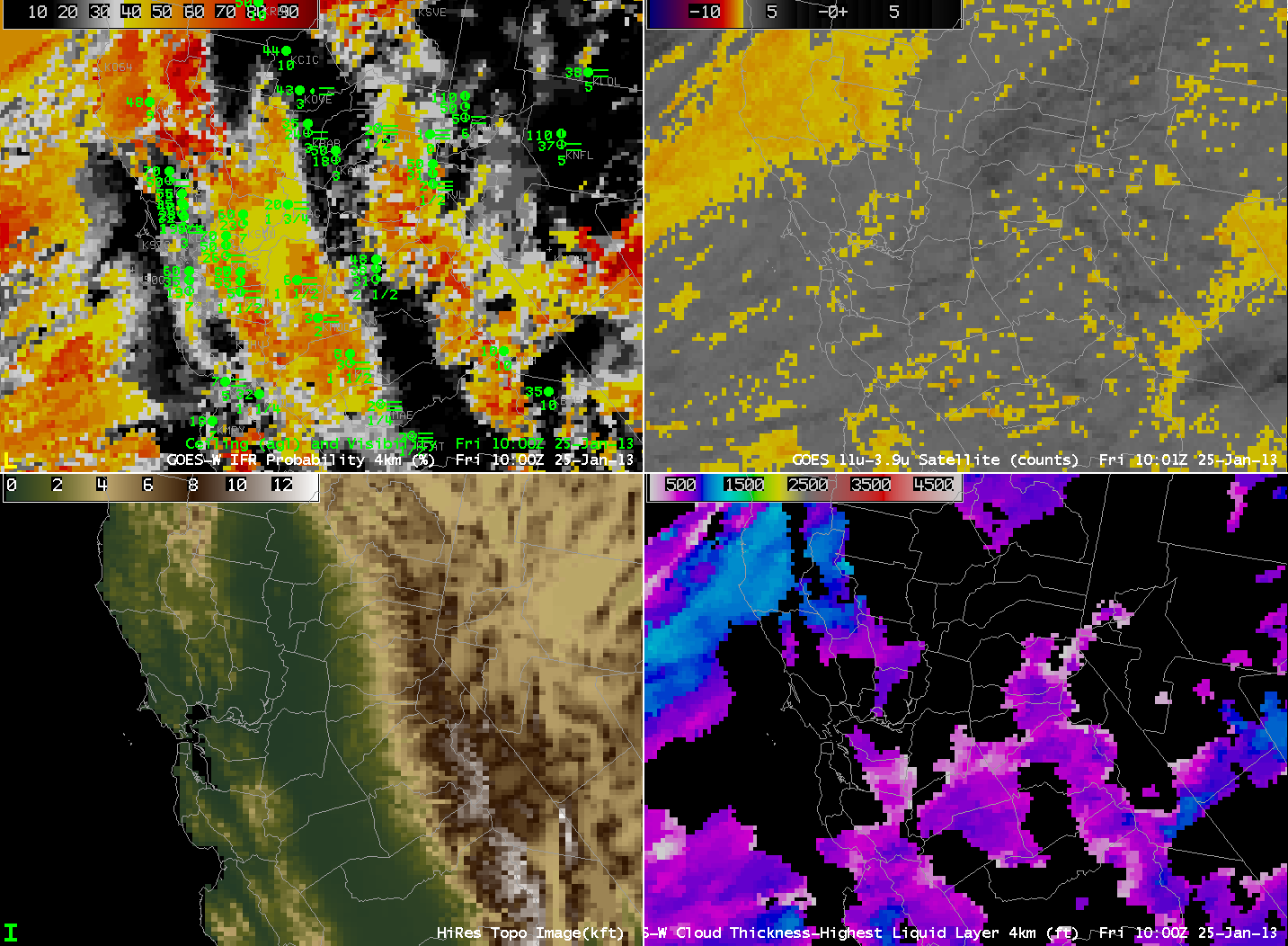
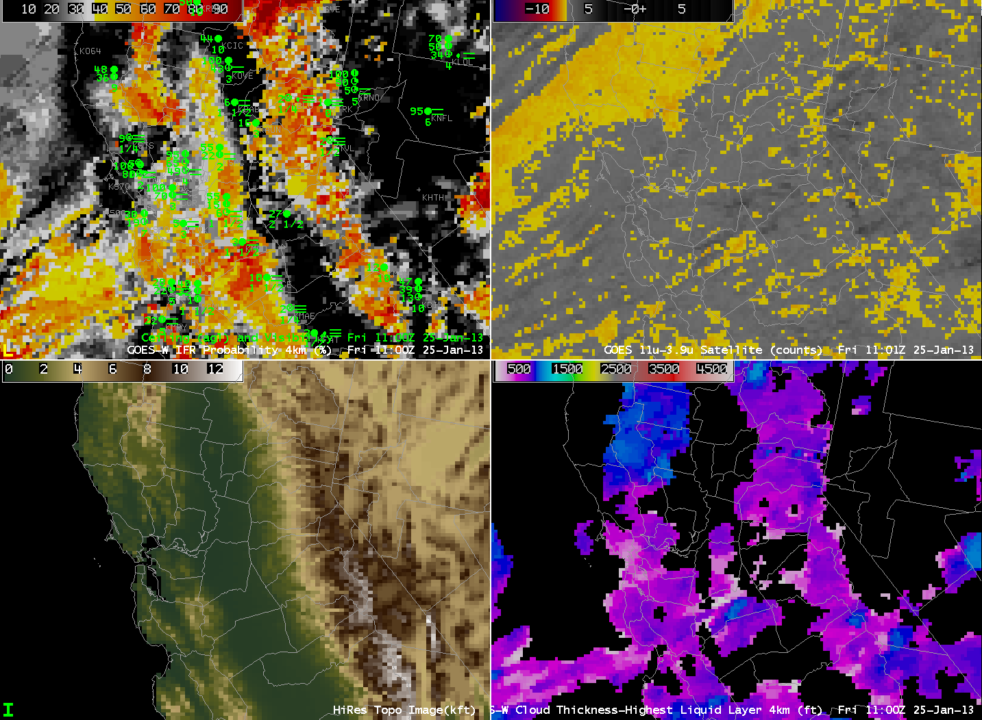
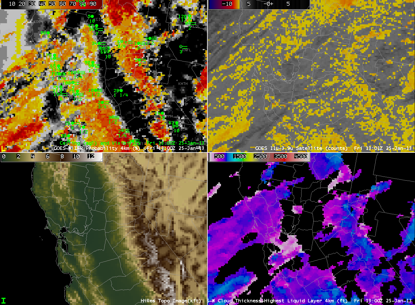
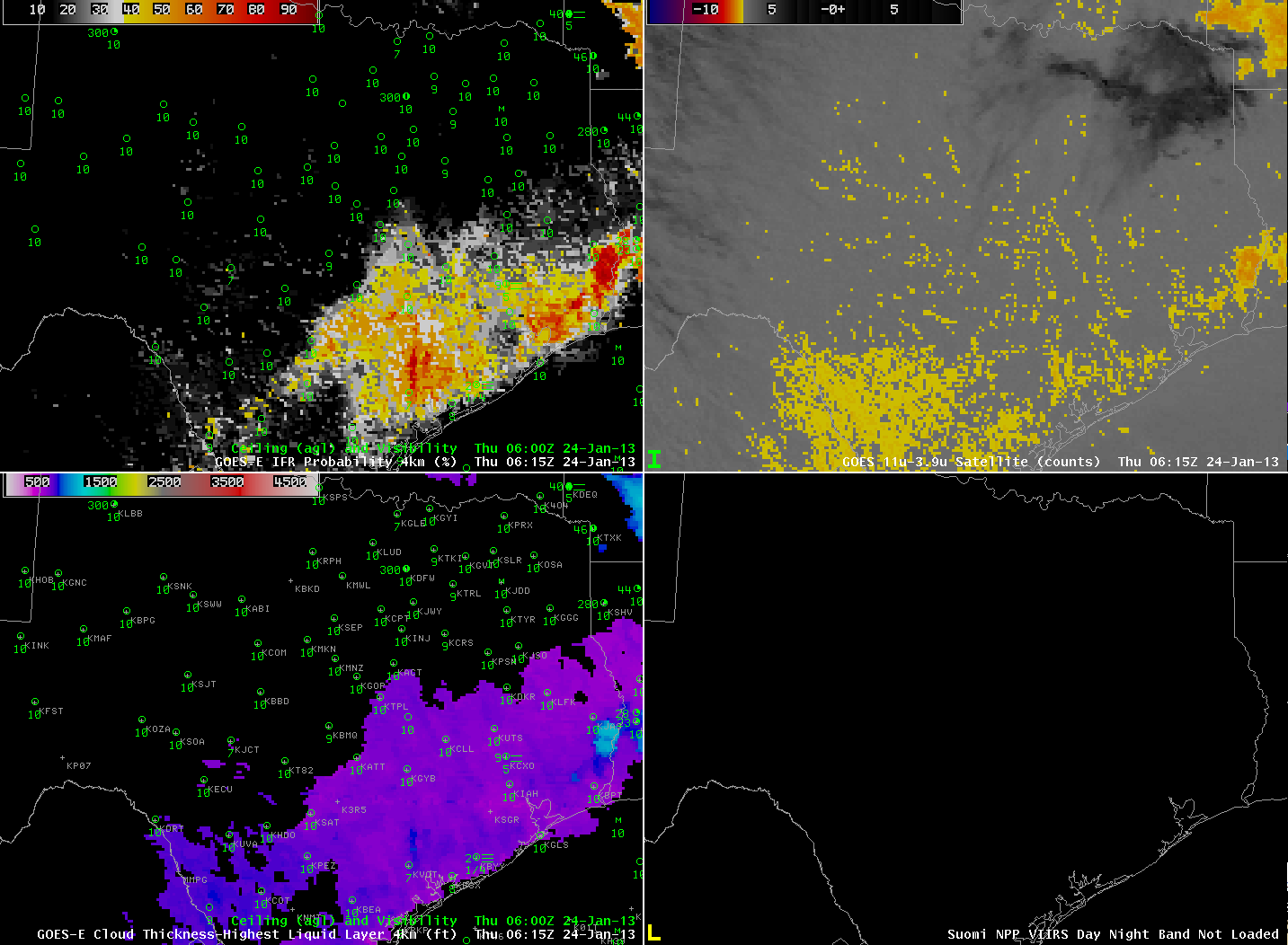
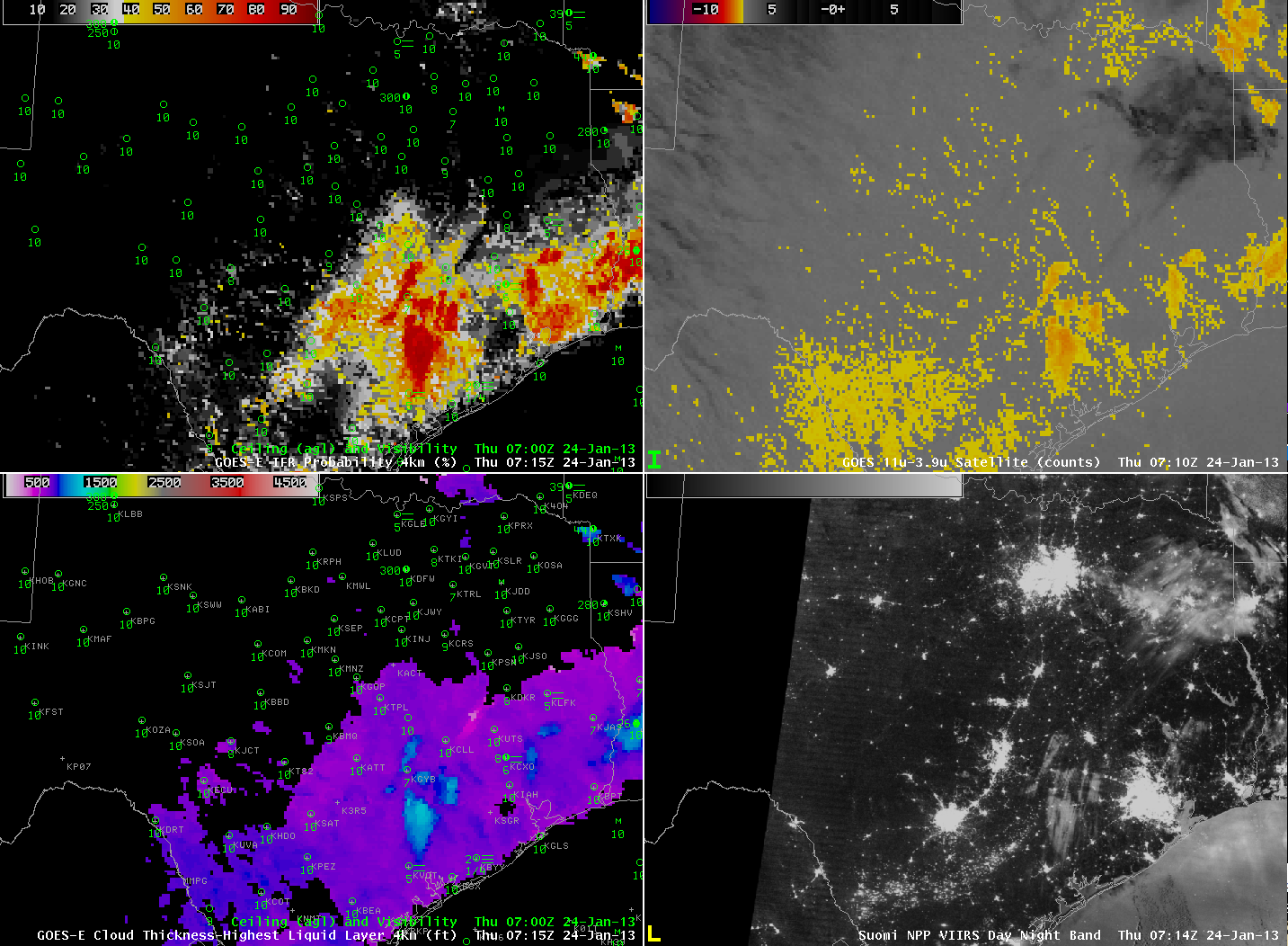
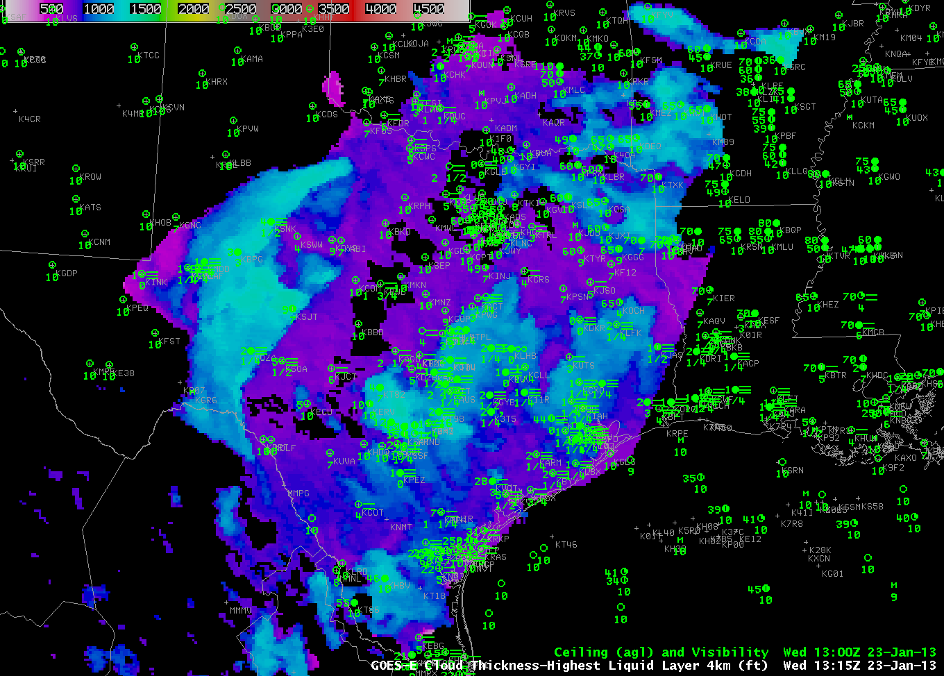
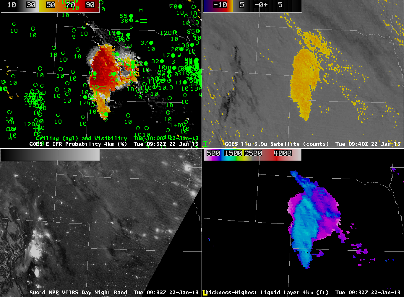
GOES-R Cloud Thickness over Arkansas just before Dawn — note that dawn has arrived over Tennessee and Mississippi

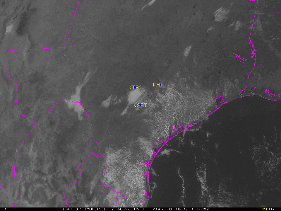
Cloud Thickness just before twilight conditions can be used to predict when radiation fog will burn off, using this scatterplot as a guide.  The maximum thickness over south-central Arkansas is 1350 feet, and that thickness corresponds to 5 hours after sunrise, or sometime after 1800 UTC.  The animation of visible imagery, below, shows that fog/low clouds are lingering over parts of southern Arkansas.

GOES-13 Visible Imagery over Arkansas, times as indicated.

California Fog

GOES-R IFR Probability computed from GOES-West (Upper Left), GOES-R Cloud Thickness computed from GOES-West (Lower Left), GOES-West Brightness Temperature Difference (10.7 µm – 3.9 µm) (Upper Right), GOES-West 10.7 µm imagery (Lower Left) at 0400 UTC 4 February

Fog develped over the San Joaquin and Salinas Valleys of California early on 4 February.  At 0400 UTC, the Brightness Temperature Difference signal shows a noisy signal over the east part of the San Joaquin Valley, with a more coherent signal off the coast and over Kern and Kings County.

As above but at 0900 UTC.

By 0900 UTC, five hours later, although the seemingly noisy signal continued over the California in the brightness temperature difference product, the GOES-R IFR probability field is starting to show higher values aligned through the San Joaquin and Salinas Valleys, where IFR conditions have developed.

As above, but at 1200 UTC

At 1200 UTC, above, high IFR probabilities extend through the Salinas Valley and in the San Joaquin valley where IFR conditions are noted.  IFR probability is also high over San Francisco Bay where marine stratus has moved inland.

As above, but at 1500 UTC

The regions of reduced visibility continue at 1500 UTC, the last image before twilight conditions disallows computation of Cloud Thickness (indeed, the terminator is apparent in the image).  The cloud thickness of 1100 feet suggests, based on this scatterplot, a dissipation time of around 4 hours.  The animation below shows visible imagery at 1730, 1830 and 1930 UTC that aligns with the predictions.

GOES-15 0.62 µm Visible Imagery, times as indicated.

Suomi/NPP VIIRS data overflew this region twice during the night, and provided brightness temperature difference information at high spatial resolution.  The GOES-R IFR algorithm is not yet applied to Suomi/NPP data (like it is to MODIS data) however.

As at top, but with Suomi/NPP Brightness Temperature Difference (10.8 µm – 3.74 µm) in the lower right, at ~0900 UTC.
As above, but at 1030 UTC.

Fog in California’s Central Valley

GOES-R IFR Probabilities (Upper Left), GOES-West Brightness Temperature Difference (10.7 µm – 3.9 µm) (Upper Right), GOES-R Cloud Thickness (Lower Left), GOES-West Water Vapor imagery (6.7 µm)

Fog developed in the early morning of February 1, 2013, in California’s Central Valley, the combination of the San Joaquin valley to the south and the Sacramento Valley to the north.  The imagery above shows the GOES-R Fog/Low Stratus product and the traditional fog product, the brightness temperature difference between 10.7 µm and 3.9 µm.  The GOES-R Product (IFR Probability) is first in highlighting the development of fog near the San Joaquin River and reductions in visibility occur in sync with the increase of IFR probabilities. The traditional GOES-West brightness temperature difference product displays considerable signal in the first hours of the animation above, but there is no organization to the signal.  Eventually, however, the brightness temperature difference signal does include the fog and low stratus in the Valley.

Multiple Cloud Layers/High Clouds over Fog

GOES-R IFR Probabilities computed from GOES-East (Upper Left), GOES-East Brightness Temperature Difference (10.7 µm – 3.9 µm) (Upper Right), GOES-R Cloud Thickness of highest liquid water layer (Lower Left), GOES-East Water Vapor (6.7 µm) (Lower Right)

It’s very common in late Winter and early Spring to have a cirrus shield over a region of dense advection fog.  The water vapor imagery, above, shows the cirrus associated with a developing warm conveyor belt over the central part of the USA.  Note how the cirrus signal also shows up in the brightness temperature difference field, and the emissivity properties of ice clouds differ strongly from those of water-based clouds (that in the enhancement in the upper right are orange versus black for ice clouds).  The presence of cirrus also precludes computation of GOES-R cloud thickness, as shown in the lower left imagery.

GOES-R IFR probabilities allow for the identification of regions of low clouds/fog even underneath the high clouds.  Note over Michigan the relatively high probabilities.  The probabilities are generated using only model-based predictors (because the satellite algorithm sees only the high clouds so satellite predictors are very small or missing).   The 1000 and 1300 UTC imagery, below, shows widespread IFR conditions underneath cirrus over Michigan and surrounding states.  IFR conditions are generally present in regions where the IFR probabilities are high.  Ceilings/visibilities do not meet IFR criteria over Western Illinois where IFR Probabilities are much lower.

As above, but centered over Michigan

Advection Fog in the Midwest

GOES-R IFR Probabilities from GOES-East, hourly from 00:15 through 13:15 on 28 January 2013, with surface visibilities and ceilings.

Warm and moist air streaming north from the southern Plains has encountered the cold (and in some places) snow-covered ground.  This is a time-honored recipe for advection fog, and the GOES-R IFR Probabilities fields, above, neatly capture the horizontal extent of the visibility restrictions overnight.  The highest IFR Probabilities occur in regions where both Satellite Predictors and Model-based predictors are high.  Note, for example, the somewhat lower probabilities that develop over Nebraska at the end of the animation.  This is a region where higher clouds are moving in.

GOES-R IFR Probabilities (Upper Left), GOES-East Brightness Temperature Difference (10.7 µm – 3.9 µm) (Upper Right), GOES-R Cloud Thickness (Lower Left), GOES-East 10.7 µm Brightness Temperature (Lower Right)

Note how the Cloud Thickness product is not computed where the higher clouds are moving in.  The product is computed only where single layer clouds are present in non-twilight conditions.  Twilight conditions are present in the eastern half of the final image, at 1315 UTC.  When radiation fog is present (rather than advection fog in this case), the last cloud thickness before twilight conditions can be used to estimate dissipation time using this chart.

GOES-R IFR Probabilities (Upper Left), GOES-East Brightness Temperature Difference (10.7 µm – 3.9 µm) (Upper Right), GOES-R Cloud Thickness (Lower Left), GOES-East Visible Imagery (0.62 µm) (Lower Right)

Holes in the advection fog developed around 1700 UTC.

IFR Conditions surround California’s Central Valley

GOES-R IFR Probabilities compted from GOES-West (Upper Left), GOES-West Brightness Temperature Difference (10.7 µm- 3.9 µm) (Upper Right), Central Valley Topography (Lower Left), GOES-R Cloud Thickness of Highest single liquid layer (Lower Right), 1000 UTC on 25 January 2013

GOES-R IFR Probabilities suggest the presence of IFR conditions both to the west and to the east of California’s San Joaquin Valley, providing a much more coherent signal of IFR conditions than can be discerned from the traditional Brightness Temperature Difference Product.  That traditional product is hamstrung by the multiple cloud layers present over the West Coast as an extratropical cyclone approaches from the Pacific Ocean.  The signal present at 1000 UTC (and earlier) continues through most of the morning.  The synthesis of Satellite Predictors and Model Predictors (Rapid Refresh Model) in the Naive Bayesian Model produces a product that gives better information in this case on exactly where IFR conditions are most likely.

As above, but at 1100 UTC

As above, but at 1145 UTC

As above, but at 1300 UTC

As above, but at 1400 UTC

Radiation Fog over Texas, Day 2

GOES-R IFR Probabilities computed from GOES-East and the Rapid Refresh Model (Upper Left), GOES-East Brightness Temperature Difference (10.7 µm – 3.9 µm) (Upper Right), GOES-R Cloud Thickness computed from GOES-East (Lower Left), Suomi/NPP VIIRS Day/Night Band (Lower Right), 0615 UTC on 24 January 2013

Clear skies and light winds again allowed for the development of radiation fog over southeast Texas.  How did the development, and the detection of fog, differ for this event from the event 1 night previous (as discussed here).  The 0615 UTC imagery, above, shows a separation between where the Brightness Temperature Difference (the heritage fog detection product) and where the GOES-R IFR probabilities are suggesting fog is present.  The Heritage Fog Product is focused on the Rio Grande Valley whereas the GOES-R IFR Probability is focused (correctly, as it turns out) on southeast Texas.  Note also that the Brightness Temperature Difference product has a signal representative of higher clouds (the dark region) over northeast Texas.

As above, but at ~0715 UTC

 At 0715 UTC, IFR probabilities are increasing over southeast Texas between Houston and San Antonio.  Suomi/NPP Day/Night band imagery at that time shows evidence of clouds in the region of highest IFR probabilities.  The traditional brightness temperature difference product continues to highlight a region near the Rio Grande Valley.

As above, but at ~0845 UTC

At 0845 UTC, IFR probabilities continue to increase over southeast Texas in the region surrounding Houston and a region near San Antonio.  The Day/Night band detects the cloudiness present in those regions.  High clouds persist over northeast Texas.

As above, but at 1315 UTC

Shortly before sunrise, fog is widespread over southeast Texas.  IFR probabilities are highest where both model and satellite predictors can be used.  Over northeast Texas, where cirrus clouds are present and where the brightness temperature difference product can therefore not provide guidance, the Rapid Refresh data are suggesting that fog is present (as observed), but IFR probabilities are lower because the satellite predictor is not used.

Radiation fog over Texas

Hourly GOES-R IFR Probabilities starting at 0345 UTC 23 January overlain with the following hour’s Ceilings/Visibilities

Light winds and clear skies over Texas promoted the development of Radiation Fog early in the morning on 23 January 2013.  The animation above shows hourly snapshots of GOES-R IFR Probabilities and observations of Ceilings/Visibilities.  IFR conditions develop first near the coast and then spread inland.  IFR probabilities neatly match the regions of observed IFR conditions.  GOES-R products also include Cloud Thickness, below, which can be used to estimate the time of Fog Dispersal.

As above but for GOES-R Cloud Thickness

The GOES-R Cloud Thickness product estimates the depth of the single-layer water cloud in non-twilight conditions, and it shows the steady deepening of the fog/low stratus overnight, with the thickest clouds occurring in the triangle between San Antonio, Fredericksburg and Austin.  The depth of the clouds just before twilight conditions can be used to estimate cloud dissipation.  The time of that image is 1315 UTC (Note that twilight conditions have already occurred in Louisiana at this time), and is shown below:

GOES-R Cloud Thickness, 1315 UTC on 23 January 2013

 Maximum values of Cloud Thickness in central Texas are 1200-1300 feet, and according to this chart, that suggests a dissipation time of more than 4 hours, or sometime after 1715 UTC.  The visible image from 1745 UTC on 23 January, below, shows a small patch of stratiform clouds remaining where the thickest radiation fog had been.

GOES-13 Visible imagery, 1745 UTC on 23 January 2013

The animation below includes the traditional fog product, the brightness temperature difference between 10.7 µm and 3.9 µm.  The GOES-R product refines the satellite estimate of fog/low stratus by using data from the Rapid Refresh Model.

GOES-R IFR Probabilities (Upper Left), GOES-East Brightness Temperature Difference (10.7 µm – 3.9 µm) (Upper Right), GOES-R Cloud Thickness (Lower Left), GOES-East 10.7 µm imagery (Lower Right)

Fog/Low Stratus over the High Plains

Surface Weather Maps, 0300, 0600 and 0900 UTC on 22 January

High Pressure with origins in the Arctic has pushed cold air into the central United States.  The western edge of the cold dome shows as a stationary front that stretches from central Kansas northwestward into Montana and beyond.  During the early morning hours of 22 January, a small region of IFR conditions developed over western Nebraska.  How did the GOES-R Fog products do in describing this region?

GOES-R IFR Probabilities and surface plots of ceilings/visibilities (Upper Left), GOES-East Brightness Temperature Difference (Upper Right), Suomi/NPP Day/Night Band (Lower Left), GOES-R Cloud Thickness (Lower Right) for various times from 0102 through 1102 UTC 22 January 2013

The animation above shows increasing IFR probabilities over southwest and west-central Nebraska over the course of the night in a region where IFR conditions are developing.  Note how the IFR probabilities are not enhanced in regions where the traditional brightness temperature difference product does have a signal — over eastern Nebraska and northeastern Kansas.  In these regions, the Rapid Refresh Model fields likely include no saturation in the lowest model layers.  Suomi/NPP Night-time Visible imagery, below, at 0752 UTC and at 0933 UTC also show the extent of the fog and low stratus.   However, it’s impossible to tell from the satellite where the visibility obstructions are most likely — that’s why the model data are important in this fused product.  Note the distinct change in illumination between 0752 UTC and 0930 UTC.  The Waxing Gibbous moon set around 0900 UTC.

As above, but for 0745 – 0800 UTC on 22 January 2013

As above, but for 0930 UTC on 22 January 2013

IFR conditions with multiple clouds layers over the southeast US

GOES-R IFR Probabilities from GOES-East (Upper Left), GOES-East Brightness Temperature Differences (Upper Right), GOES-R Cloud Thickness (Lower Left), Surface Observations of Ceilings and Visibility (Lower Right), all at 1000 UTC on 16 January 2013

A slowly-moving weather system brought extensive cloudiness and IFR and near-IFR conditions over the southeast part of the United States again on January 16, and provided a good example of how the fused nature of the GOES-R Fog/Low Stratus product — combining both satellite and model information — yields a better signal (than is available from the traditional brightness temperature difference product) of where fog and low stratus are most likely.  The imagery from 1000 UTC, which is characteristic of the entire event, shows a brightness temperature difference signal over the southest that is consistent with the observed multiple cloud layers.  Such a cloud configuration makes it very difficult to relate the brightness temperature difference signal to surface observations.  in contrast, the IFR Probability field show a widespread region of high probabilities, overlapping the regions of near-IFR and IFR observations over Tennessee, and points south.  Cloud thickness, which is computed only where single water-cloud layers are detected from satellite, indicates cloud thicknesses around 1000 feet.  Note that where the cloud thickness is diagnosed, in general, IFR probabilities are relatively larger.  This is because IFR probabilities combine satellite predictors and model predictors.  If the satellite predictors cannot be generated because of multiple cloud layers and/or a single high cirrus deck, then only the model predictors are driving the IFR probability value, and the probability will therefore be lower.  This is the case over western Tennessee and central Georgia.