Category Archives: New England

Fog over southern New England

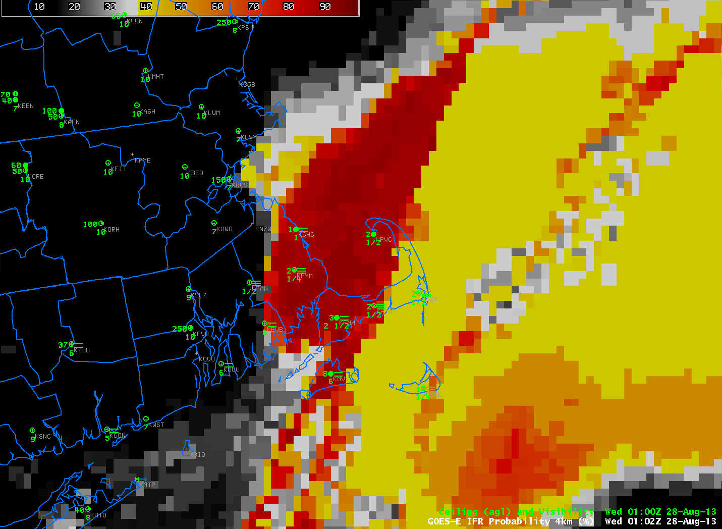
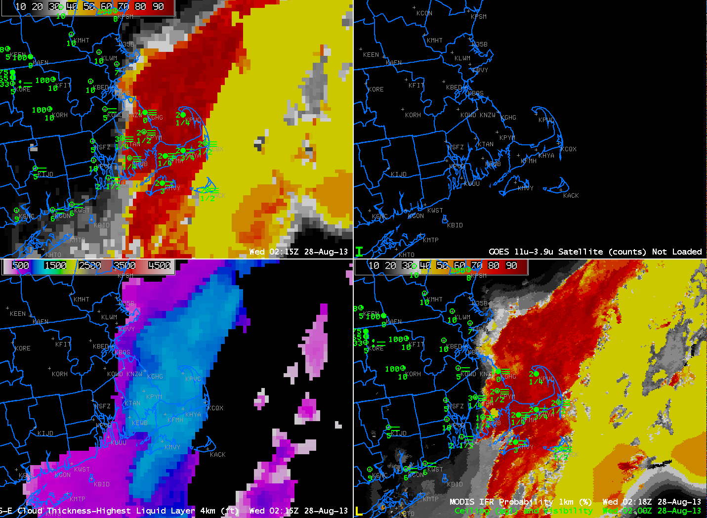
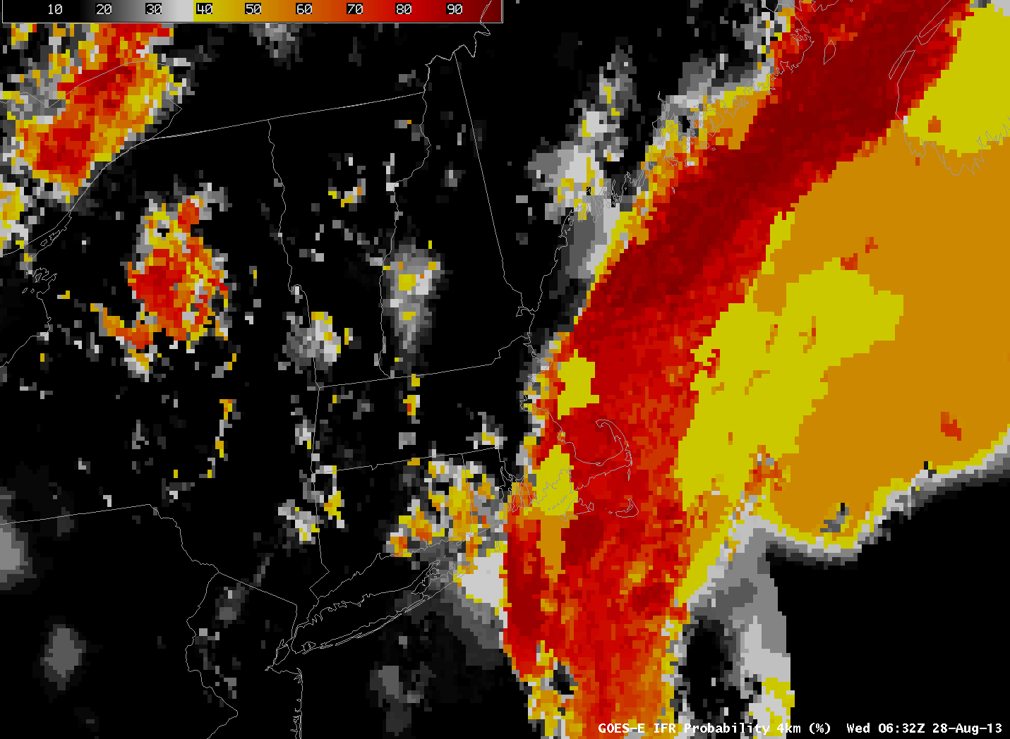
The National Weather Service in Taunton, MA, tweeted an image of fog over coastal southern New England early on September 3rd. How well did the GOES-R IFR Probability detect this event?

GOES_IFR_PROB_20130903loop

GOES-R IFR Probability (click image to play animation)

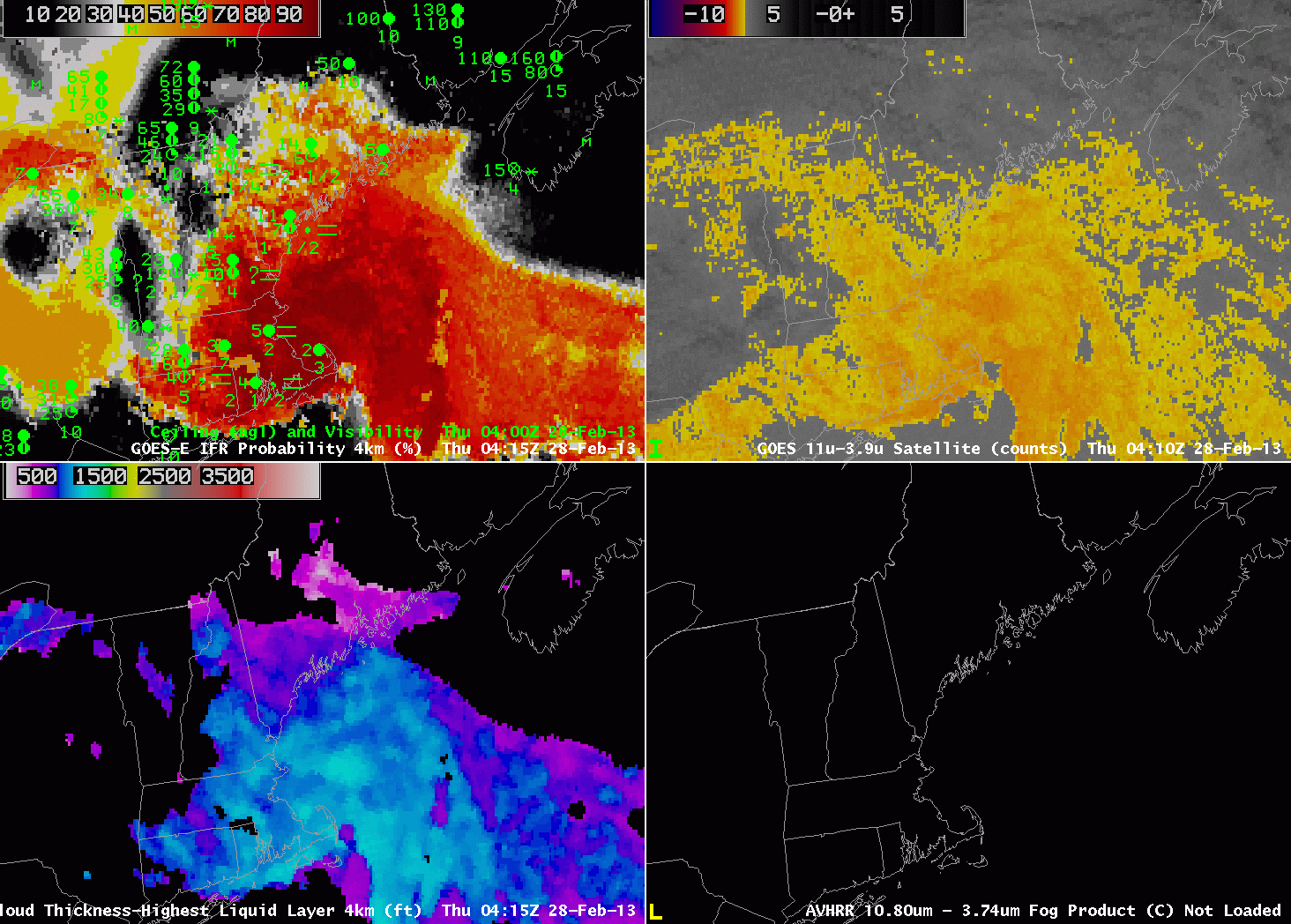
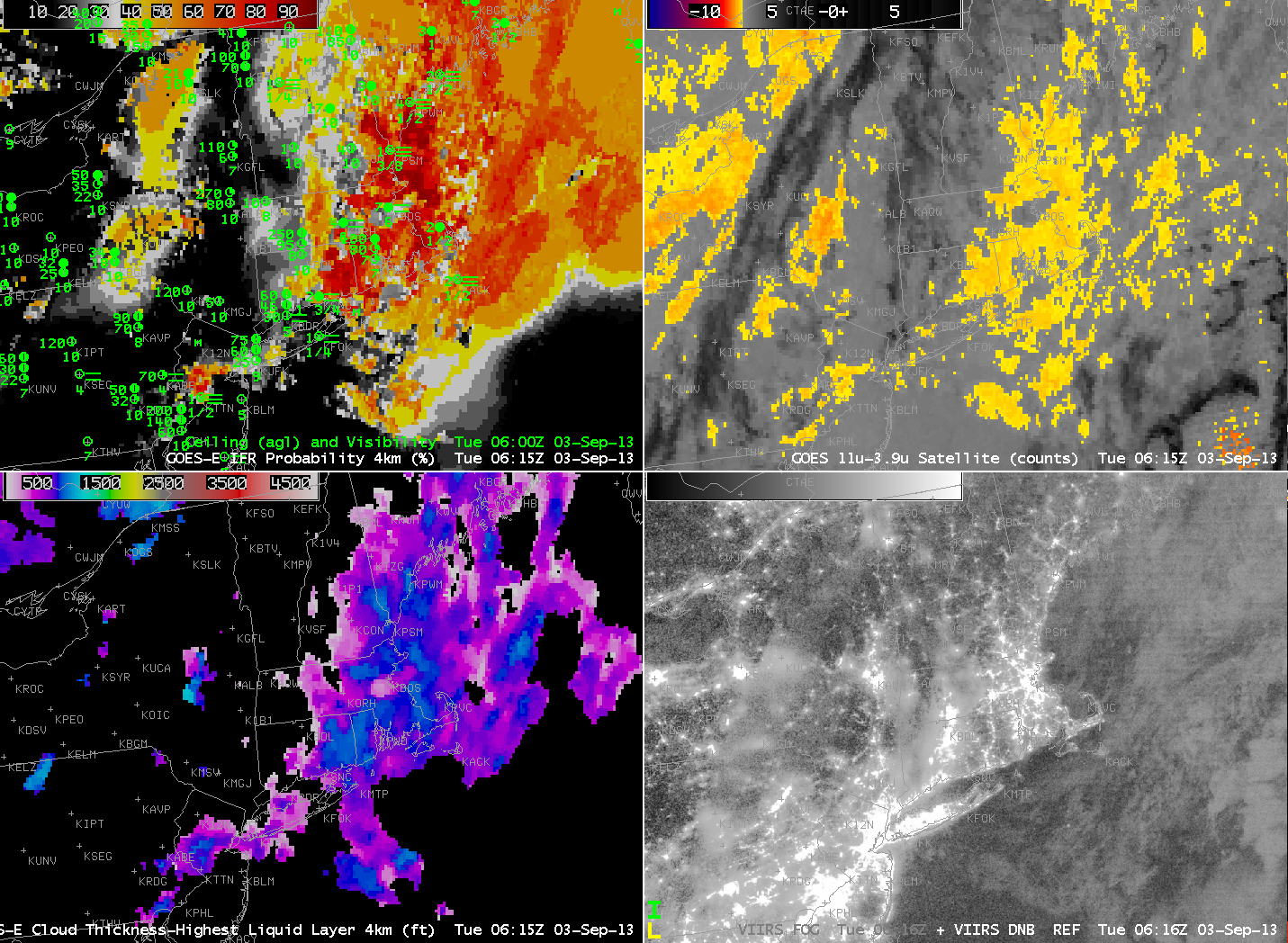
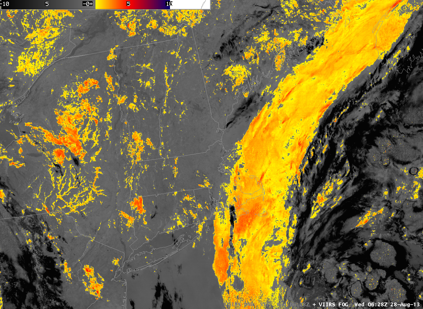
The animation, above, at hourly time-steps (GOES-R IFR Probability is computed every 15 minutes, usually, but matching surface observations occur only hourly) can be used to validate the accuracy of the IFR Probability product: highest probabilities in the animation are occurring over coastal New England where visibility is lowest. The increase in probabilities from 1002 UTC to 1102 UTC over the Gulf of Maine reflects the night-time (1002 UTC) vs. daytime (1102 UTC) predictors being used in the IFR Probability algorithm. The flat nature of the IFR probability field over parts of the Gulf of Maine suggests that model data only is being used to compute the IFR probability field there. This occurs where high clouds obscure the satellite view of low clouds.

GOES_IFR_PROB_20130903_1315loop

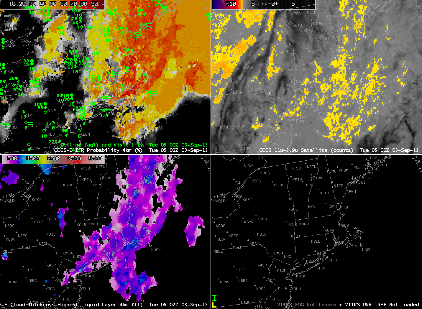
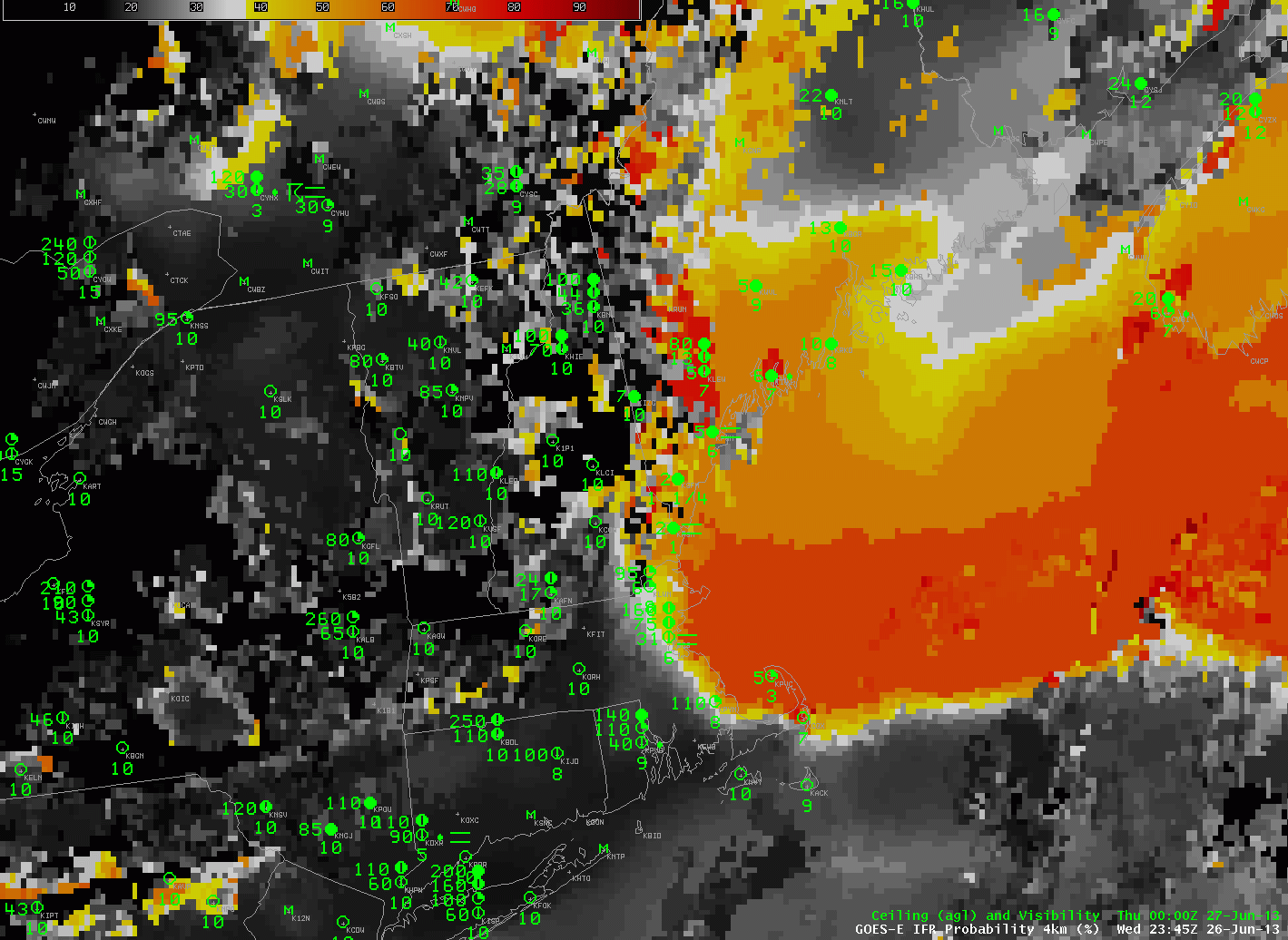
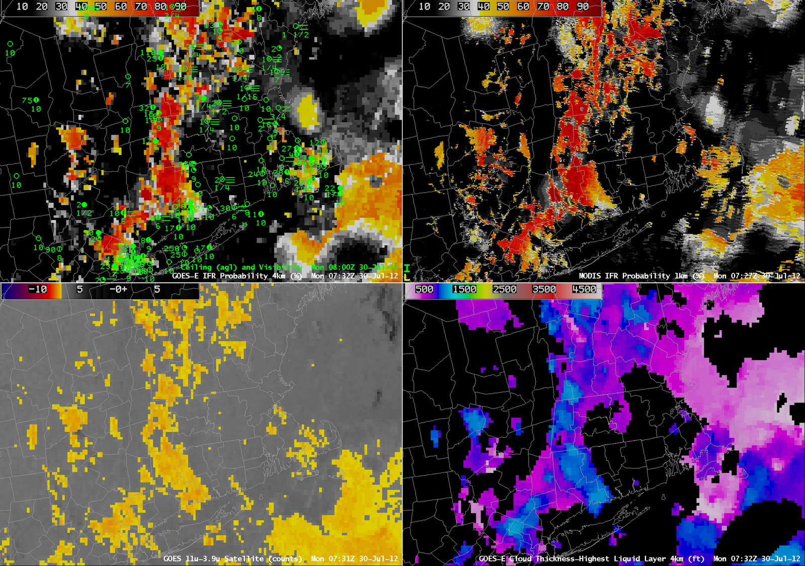
GOES-R IFR Probability (Upper Left), GOES-East Brightness Temperature Difference (Upper Right), GOES-R Cloud Thickness (Lower Left), Suomi/NPP Day/Night Band (Lower Right) (click image to play animation)

The brightness temperature difference fields in the animation above (click image to see the animation) have a characteristic appearance associated with high clouds south and east of Cape Cod. In fact, Nantucket is mostly overlain by high clouds. The presence of those high clouds makes satellite detection of fog/low stratus difficult, but a fused/blended product such as the GOES-R IFR probability field that combines satellite and model data is able to alert an observer to the presence of reduced visibilities.

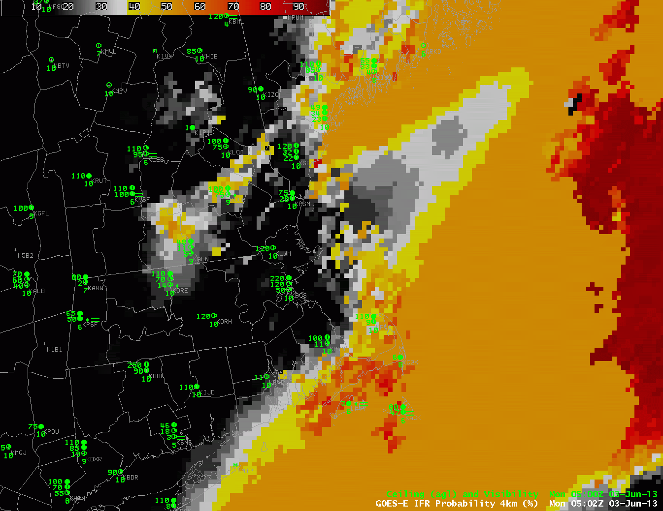
The GOES-R Cloud Thickness (Lower left in the animation above) gives an estimate to the depth of the highest water-based cloud layer. This product is not computed during twilight conditions — from about 1015 to 1215 UTC in the animation above. The animation clearly shows the thickest fog/low stratus deck moving eastward through southeast New England during the early morning hours.

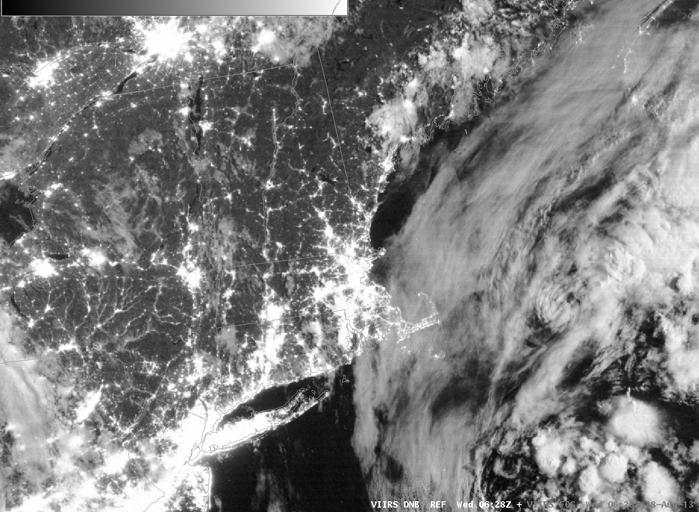
The Suomi/NPP Day/Night band allows for visible imagery at night, detecting visible moonlight and Earthglow that is reflected off clouds, and also emitted light from cities. The 0615 UTC image is here. Clouds are visible in the image, but there is no information on the level of the cloud.

GOES_EAST_3SEP2013loop

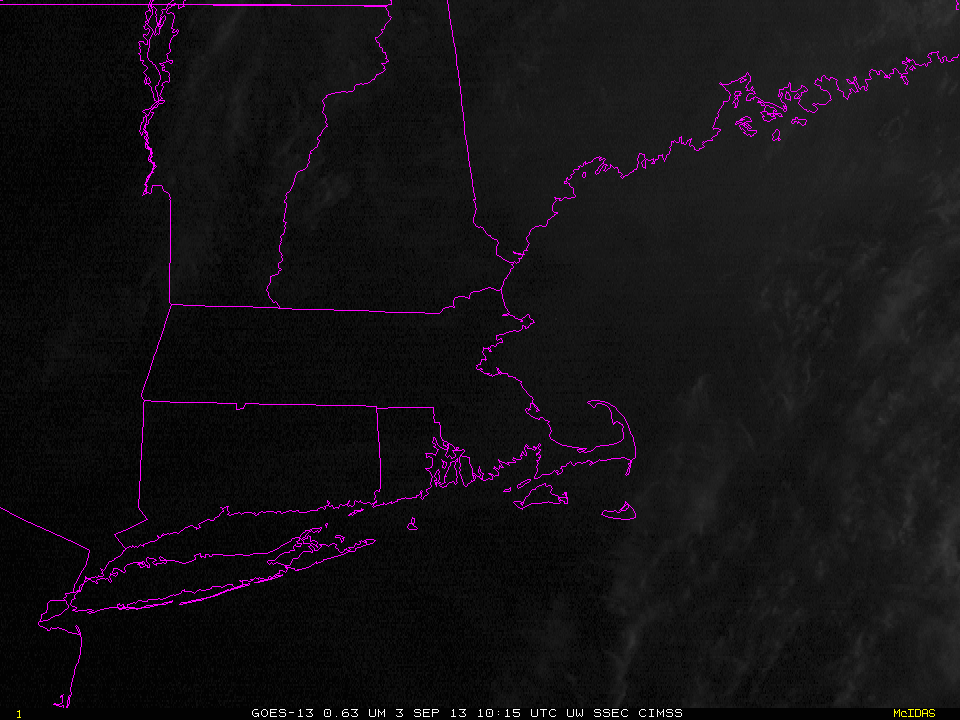
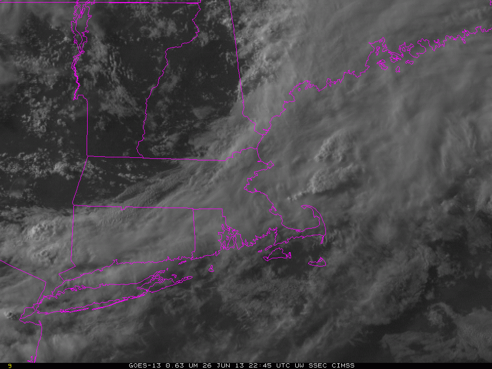
GOES-13 Visible Imagery (click image to play animation)

Visible imagery from after sunrise shows the low clouds persisting south of New England. In addition, a bore (manifest as a series of parallel lines) propagates south of an area of convection that appears to have spawned the bore.

Fog on Cape Cod

Loop of IFR Probabilities

Fog developed over Cape Cod and the Islands overnight into the early morning on August 28th. The animation above (click image to animate) shows high IFR probabilities over land adjacent to the ocean. Observations show IFR or near-IFR conditions in these regions. IFR conditions decreased after sunrise. By 1410 UTC, the final image in the loop, IFR conditions persisted mostly only over Nantucket and Cape Cod east of Falmouth. This is where highest IFR probabilities persisted. The GOES-based IFR Probabilities suggest a sharp edge to the lowest visibilities over far eastern Massachusetts, which edge was just east of a Newport (RI) to Taunton (MA) line. MODIS-based IFR probabilities at 0218 UTC, below, also suggest a sharp western edge to the IFR conditions.

MODIS-based IFR Probabilities

VIIRS data from Suomi/NPP includes both the Day/Night Band and a Brightness Temperature Difference. These data are toggled with the GOES-based IFR Probabilities below. Resolution limitations inherent with GOES data preclude the accurate detection of fog in small river valleys.

Suomi/NPP Day/Night Band Imagery, Brightness Temperature Difference Imagery, and GOES-Based IFR Probabilities, all near 0630 UTC on 28 August

IFR Probability Fields capture back-door cold front in New England

Visible imagery around 0000 UTC on 27 June 2013 showing the slow advance of a backdoor coldfront over eastern New England.  The yellow arrows at the end highlight the front over New Hampshire.

A back-door coldfront moved westward through New England late in the day on June 26th, bringing with it cooler air and lowered ceilings.  How well did the IFR Probability field capture the low ceilings that came with the cooler air?

GOES-R IFR Probability fields computed from GOES-East, hourly from 2345 UTC on 26 June to 0445 UTC on 27 June.

Intially (2345 UTC), high probabilities of IFR conditions were limited to the cold waters east of New England. This is reasonable given the high dewpoints (upper 60s Fahrenheit) that prevailed New England on the 26th.  Light westerly winds would move that moist air over the cold Gulf of Maine, and advection fog would form.  As the backdoor front moved across the region, IFR probabilities increased as visibilities declined.  The animation of the IFR probability fields captures the leading edge of the maritime air.

Advection fog over the Northeast as a front moves through

GOES-R IFR Probabilities, hourly, from 0500 UTC through 2002 UTC 3 June 2012

A cold front moving through eastern New England has drawn 60-degree dewpoints into that region of the country.  When that moist air then moves over the cold shelf waters and cold waters of the Gulf of Maine, fog and low stratus develop.  The GOES-R IFR Probability Field ably captures the regions of restricted visibility over coastal and offshore New England.  It also depicts the sharp northern edge of the restricted visibilities over Connecticut and Rhode Island.  The IFR probability field in the animation above is derived mostly from model data;  this is evident from the smooth nature of the field.  There are regions that are more pixelated within the smooth field.  These are regions where holes in the high cloud field associated with the front allow the satellite to see low water-based clouds.

IFR conditions in Maine

GOES-R IFR Probabilities computed from GOES-East (Upper Left), GOES-East Brightness Temperature Difference (10.7 µm – 3.9 µm) (Upper Right), GOES-R Cloud Thickness (Lower Left), Toggle between Suomi/NPP Brightness Temperature Difference (10.8 µm – 3.74 µm) and Day/Night Band “Nighttime Visible” imagery (Lower Right), all around 0815 UTC on 28 February

Weak Low pressure in the Gulf of Maine helped generate IFR conditions over the northeastern United States early in the morning on 28 February 2013.  The brightness temperature difference fields over New England from Suomi/NPP include very sharp cloud edges (also present in the Day/Night band imagery).  Because the GOES-R IFR Probability field also includes information from the Rapid Refresh, it is better able to distinguish fog and low stratus, as present over most of Maine, from elevated stratus, present over western New Hampshire and Quebec.

GOES-R IFR Probabilities computed from GOES-East (Upper Left), GOES-East Brightness Temperature Difference (10.7 µm – 3.9 µm) (Upper Right), GOES-R Cloud Thickness (Lower Left), Suomi/NPP Brightness Temperature Difference (10.8 µm – 3.74 µm) (Lower Right), times as indicated

The animation of the imagery, above, demonstrates how the GOES-R IFR probability product can be used to monitor the evolving nature of a low cloud field.  As the low pressure system in the Northeast starts to move away, the fog/low clouds rotate eastward.   Two noteworthy events in the loop are present.  The 0515 UTC imagery (mislabeled as 0510 UTC), contains stray light in the 3.9 µm field, and the traditional GOES brightness temperature difference field is therefore changed significantly, but the GOES-R IFR probability field is not.  Note also that multiple cloud layers exist over coastal Maine and New Hampshire at the end of the animation, but GOES-R IFR probabilities correctly maintain high probabilities in a region where IFR conditions are present and where the traditional brightness temperature difference field does not show a signal consistent with low clouds.

Interpreting IFR Probability Fields

Toggle between GOES-R IFR Probabilities computed from GOES-East, 0800 UTC on 30 January 2013, and the Brightness Temperature Difference from GOES-East (10.7 µm – 3.9 µm) also from 0800 UTC on 30 January 2013

The two images looping, above, show two different schemes used to detect fog and low stratus.  The one that highlights mostly land over New England is the GOES-R Fog/Low Stratus product, and it shows mostly uniform probabilities over southern New England, with a patch of higher probabilities in central Massachusetts and over southern Maine.  In contrast, the Brightness Temperature Difference Product — the traditional method of detecting fog — highlights a large area over the ocean (as well as a region in central Massachusetts that stretches southeastward to Block Island).  Note that the regions of IFR conditions are over land.  The offshore islands, and Cape Cod, do not show IFR conditions even though the heritage fog detection product has a strong signal offshore.

GOES-R IFR Probabilities are highest in central Massachusetts.  This is where both predictors — the Rapid Refresh Data and the satellite data — strongly indicate the presence of fog and low stratus.  The interpretation that should be given where roughly homogenous regions of IFR probability surround a region of higher, more variable IFR probability, as is happening in central Massachusetts, is that higher clouds (or multiple cloud layers) have parted over the region of highest IFR probabilities, allowing the satellite signal to be a factor.  This would also be a region where GOES-R Cloud Thickness could be computed.   In regions offshore, IFR probabilities are low despite the strong satellite signal becaure the Rapid Refresh data is not modeling (properly) atmospheric conditions conducive to IFR conditions.

GOES-R Probabilities are too low: Why?

GOES-R IFR Probabilities (upper left), GOES-East Visible imagery (upper right), Brightness temperature difference between 10.7 and 3.9 micrometers (lower left), GOES-R Cloud Thickness (lower right)

The imagery above shows high IFR probabilities over western Massachusetts — where IFR conditions are not observed — and very low probabilities in central Massachusetts in and near the Connecticut River Valley where IFR conditions are observed.  The brightness temperature difference in central Massachusetts is not suggestive of low clouds and fog.  For the IFR probability to be high there, then, would require that the Rapid Refresh Model showed saturation in the lower part of the model atmosphere.  Thus, the fused product could show higher probabilities in this region where fog is observed.  However, as shown below, relative humidity in the lowest part of the model was actually a relative minimum over central Massachusetts.

Two-hour forecasts of Relative Humidity from the Rapid Refresh, all valid at 0600 UTC from the 0400 UTC model run;  Lowest 30 mb of the model (upper left), lowest 60 mb of the model (upper right), lower 90 mb of the model (lower left), surface (lower right)
Two-hour forecasts of Relative Humidity from the Rapid Refresh, all valid at 0800 UTC from the 0600 UTC model run;  Lowest 30 mb of the model (upper left), lowest 60 mb of the model (upper right), lower 90 mb of the model (lower left), surface (lower right)

By 0730 UTC, the satellite brightness temperature difference product (below) is starting to suggest that fog/low clouds are more widespread (A MODIS image at the same time tells the same tale).  As that happens, the IFR probabilities start to increase.

GOES-R IFR Probabilities computed from GOES-East imager data (upper left), GOES-R IFR probabilities computed from MODIS data (upper right), Brightness temperature difference between 10.7 and 3.9 micrometers (lower left), GOES-R Cloud Thickness (lower right)
GOES-R IFR Probabilities (upper left), GOES-East Visible imagery (upper right), Brightness temperature difference between 10.7 and 3.9 micrometers (lower left) at 1032 UTC, GOES-R Cloud Thickness (lower right) not shown because of twilight conditions

The 1032 UTC imagery (above) shows the very small scale of this fog feature that is in central Massachusetts.