Category Archives: Multiple Cloud Layers

Fog over Nebraska under high clouds

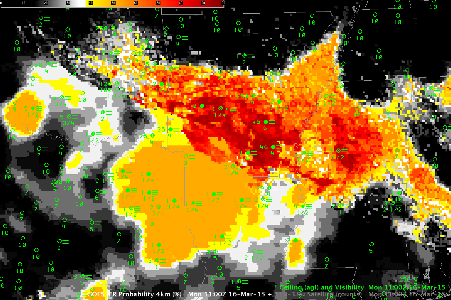
GOES-R IFR Probabilities, 0315-1215 UTC, 5 May 2015 (Click to enlarge)

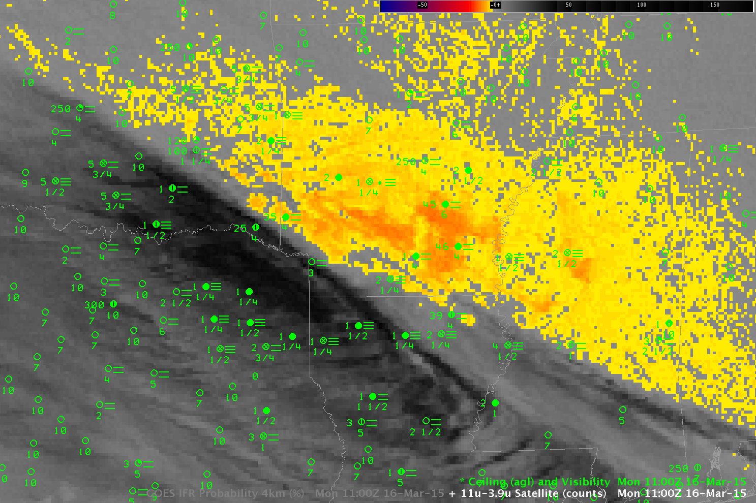
Dense Fog developed over the Hastings, Nebraska WFO overnight, leading to the issuance of Dense Fog Advisories. The GOES-R IFR Probabilities, above, show a steady increase in probabilities over the night as the fog develops. The relatively flat nature of the IFR Probability field is characteristic of GOES-R IFR Probabilities that do not include information from satellite (that is, only model fields are being used here to educe IFR probabilities). IFR Probability fields are a fused product, typically blending information from model fields and from satellite data. However, this was a case of fog developing under an extensive cirrus shield so that satellite data were not used as a predictors. The 10.7µm – 3.9µm Brightness Temperature Difference field, shown below, gives no information about surface conditions. That the IFR Probability fields neatly overlap the region of developing IFR conditions is testimony to the accuracy of the model field in simulating the lower part of the troposphere.

When only model data are used, as above, features in the field that are parallel to surface topography contours can become evident in the GOES-R IFR Probability fields. This is related to interpolation of the lowest 1000 feet of model relative humidity fields (moisture information that is used as a predictor in the computation of the IFR Probability) in regions of sloping topography.

In the animation above, note that the IFR Probabilities increase in the final frame. Over most of the scene, at 1215 UTC, the sun has risen and Daytime Predictors are being used to compute IFR Probabilities. (The dividing line between Daytime — to the east — and nighttime — to the west — is visible stretching north-northwest to south-southeast from the extreme northeast corner of Colorado). IFR Probabilities are somewhat higher during the day (compared to night) because visible imagery is incorporated into the satellite predictors; more accurate cloud clearing means that IFR Probabilities increase just a bit.

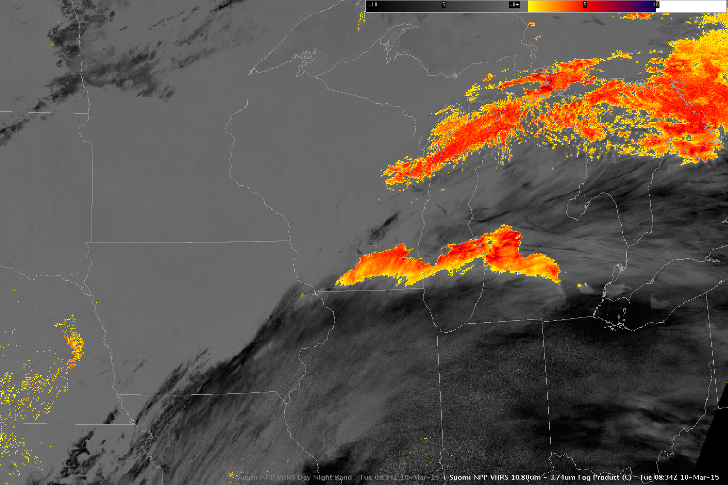
GOES-13 Brightness temperature difference fields (10.7 µm – 3.9 µm) over the Great Plains, 0630-1300 UTC, 5 May 2015 (Click to enlarge)

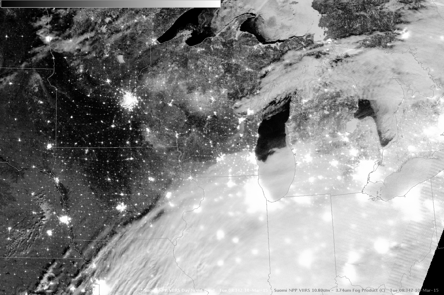
Suomi NPP overflew Nebraska, giving a view of the extensive cirrus shield. The Day Night Band gave crisp imagery as the Moon was very nearly full.

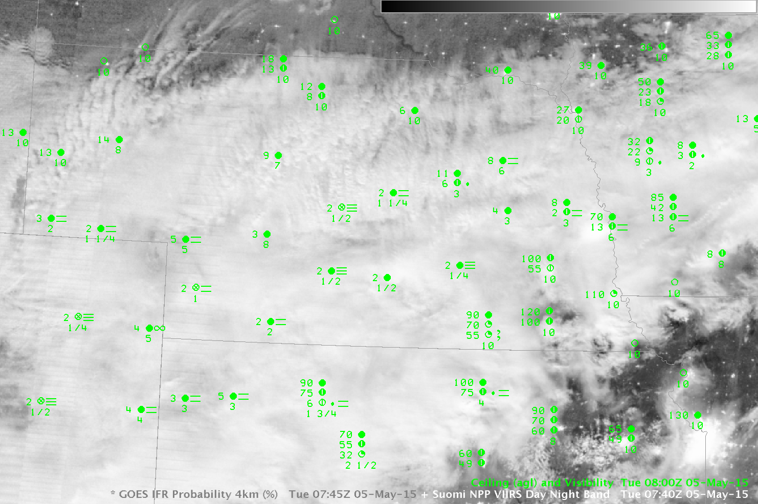
Suomi NPP Day Night Band Visible Imagery (0.70 µm) at 0740 UTC on 5 May 2015 (Click to enlarge)

Cirrus and IFR Conditions over south Texas

GOES-13 Brightness Temperature Difference (10.7µm – 3.9µm) Fields, 0100-1400 UTC on 25 March 2015, along with surface observations of ceiling and visibility (Click to enlarge)

GOES-13 Brightness Temperature Difference Fields, above, demonstrate how high and middle clouds can complicate or prevent the detection of low clouds from satellite. The beginning of the animation shows signatures of cirrus streaking across the northern part of the domain. There are also signals of low clouds/fog over south Texas that diminish by ~0300 UTC before reappearing. No fog is reported during the early part of the animation. In the latter half of the animation, cirrus moves in to the southern part of the domain from the southwest (cirrus appears black in the enhancement used), interfering with the detection of low clouds and fog over south Texas. At 1400 UTC, the end of the animation, reflected 3.9µm radiation originating from the rising sun has flipped the sign of the brightness temperature difference field.

GOES-13-based IFR Probability Fields, 0100-1400 UTC on 25 March 2015, along with surface observations of ceiling and visibility (Click to enlarge)

The GOES-R IFR Probability fields, above, show little signal until after 0500 UTC when the satellite and model data both start to suggest the presence of fog/low stratus. When the cirrus impinges on the southern part of the domain, becoming noticeable at 1000 UTC, IFR Probability values drop because satellite predictors cannot be used in the algorithm — only model data is driving the field over south Texas. The model data strongly suggests fog is present however (and IFR and near-IFR conditions are reported). Using the fused product allows a forecaster to have a consistent signal as the high clouds move in. IFR conditions persist — and IFR Probabilities remain high — after sunrise over portions of south Texas.

Fog under high clouds

Early morning March 16 2016 had another fine example of the importance of using fused information to detect regions of low clouds and fog. The animation above shows the Brightness Temperature Difference (10.7µm – 3.9µm) and IFR Probability fields from 1100 UTC 16 March 2016. A cirrus canopy over Texas and Louisiana prevents the satellite from detecting radiation emitted from lower clouds. In this region, the IFR Probability field can suggest the presence of fog/low stratus and IFR Conditions because of low-level saturation that is present in the Rapid Refresh Model. Fusing this information together allows for a better depiction of where IFR Conditions are present. Cirrus clouds are not present over Arkansas; there, both satellite and model can be used to compute IFR Probabilities. When both satellite and model suggest fog is present, IFR Probabilities are higher (over Arkansas) than when only model (over Louisiana), or only satellite, suggest fog is present.

Fog under high clouds over the Midwest

GOES-R IFR Probability Fields, 0200-1100 UTC on 10 March 2015, along with surface observations of ceilings and visibilities (Click to enlarge)

A region of dense fog/low clouds moved northward overnight through Illinois and into Wisconsin. Its movement northward was captured accurately by the GOES-R IFR Probability fields, above. IFR conditions develop as the region of high IFR Probability moves overhead. In addition, as the IFR Probability fields move northward, ceilings and visibilities along its southern flank improve. That is, the IFR Probability fields capture the northward motion of improving visibilities over Illinois. Detecting when visibilities improve is as important as detecting when visibilities deteriorate, and the GOES-R IFR Probability field in this case is doing both.

Compare that to the traditional method of detecting low clouds, the brightness temperature difference field, shown below. Low stratus and fog along the northern edge of the cirrus shield is detected, but the northward movement of the southern edge of the IFR conditions cannot be detected under the cirrus.

GOES-East Brightness Temperature Difference Fields (10.7µm – 3.9µm), 0700-1100 UTC, 10 March 2015 (Click to enlarge)

Suomi-NPP overflew the region at 0830 UTC, just as the fog was moving into southern Wisconsin. The image below shows the extensive cloud field. The brightness temperature difference field (11.32µm – 3.74µm) (here) for the same time suggests that much of the cloudiness detected over Illinois is higher cloud.

Suomi NPP Day Night Band (0.70 µm) imagery, 0334 UTC on 10 March 2015 (Click to enlarge)

IFR Conditions over the Southeast United States

Brightness Temperature Difference Fields (10.7µm – 3.9µm) from GOES-East, hourly from 0400-1300 UTC on 2 March 2015 (Click to enlarge)

A series of frontal systems along the east coast caused multiple cloud layers and IFR conditions over much of the deep south and piedmont from Mississippi to Georgia and up through Virginia overnight on 1-2 March 2015. The animation of Brightness Temperature Difference (10.7µm – 3.9µm), above, is testimony to the difficulty in using that product as a fog detection device when multiple cloud layers are present: Many stations underneath cirrus show IFR Conditions. (Note also how the signal changes at 1300 UTC — the end of the animation — as the sun rises and increasing amounts of 3.9µm solar radiation is reflected off the clouds).

The GOES-R IFR Probability fields, below, better identify regions of reduced visibility underneath mixed cloud layers. It does this by incorporating model data (from the Rapid Refresh) into its suite of predictors. Thus, where low-level saturation is indicated under multiple cloud layers, IFR Conditions can be assumed to be occurring, and computed IFR Probabilities are large. The hourly animation of GOES-R IFR Probability, below, shows a good overlap between large IFR Probabilities and IFR (or near-IFR conditions). The flat IFR Probability field that is widespread over the Piedmont region of the Carolinas is typical of an IFR Probability field determined mostly by model output. Where high clouds break, pixelated regions develop (and IFR Probabilities increase) in the field.

GOES-R IFR Probability fields, 0400-1300 UTC on 2 March (Click to enlarge)

The 1215 UTC and 1300 UTC imagery in the IFR Probability animation above include a discernible nearly north-south line. (The 1215 UTC image is below). This is the terminator. To the right of that line, where IFR Probabilities are slightly larger (dark orange), daytime predictors are being used; to the left of that line, IFR Probabilities are slightly smaller (lighter orange) and nighttime predictors are being used. Why is the probability a bit larger in the daytime predictors? In part this is because visible imagery can be used to ascertain whether clouds are present. You can be a bit more confident that IFR conditions are present because clouds are present in the visible imagery.

GOES-R IFR Probability fields, 1215 UTC on 2 March (Click to enlarge)

South Texas Fog and low stratus

GOES-R IFR Probabilities, half-hourly from 0045 UTC to 1215 UTC on 4 February 2015, along wtih surface reports of ceilings and visibilities (Click to enlarge)

Fog developed over south Texas during the morning of 4 February. How did the GOES-R IFR Probability Products perform for this example, and what can be learned from them? There are at least two distinct regions in the animation above. Over much of southeast Texas, the IFR Probability field suggests multiple cloud layers are present. IFR Probabilities are smaller here because satellite-based cloud information cannot be used in the algorithm in regions where high/mid-level clouds preclude a satellite’s view of low stratus and fog. It is important to interpret the IFR Probability fields with knowledge of the cloud levels that are present. Towards the middle of the loop, fog develops in/around Midland over the high Plains. IFR Probabilities are large there because satellite data are used as a predictor because high clouds are not impeding the satellite’s view of the developing region of fog/stratus. Brightness Temperature Difference Fields from GOES, below, show the difficulty in using that field to detect fog/low stratus in regions where multiple cloud layers exist. There are many stations underneath high clouds that have undetectable (via satellite) IFR conditions.

GOES-13 Brightness Temperature Difference (10.7µm – 3.9µm), 0245 – 1215 UTC 4 February 2015 (Click to enlarge)

Toggle between GOES-based and MODIS-based IFR Probabilities at 0915 UTC on 4 February 2015 (Click to enlarge)

MODIS data from Aqua can also be used to compute IFR Probabilities, as shown above. In general, there is very good agreement between GOES and MODIS-based fields, but there are some very interesting differences along the limb of the MODIS scan in central TX where GOES data shows smaller values of IFR Probabilities than is shown in the MODIS fields — for example at San Angelo (KSJT), Kirksville (KCOM) and Brady (KBBD). This occurs in a region where limited observations show near-IFR conditions. The higher values along the limb of the MODIS scan are likely due to limb brightening that arises because the radiation being detected comes from a path that traverses more of the (colder) upper atmosphere. The affect is wavelength-dependent, and thus will show up in a brightness temperature difference field as a stronger signal, and that stronger signal will influence the IFR Probability fields. In short: interpret MODIS IFR Probability fields along the edge of the MODIS swath with this knowledge of limb effects.

Brightness Temperature Difference (11.35 µm – 3.74 µm) from Suomi NPP at 0729 and 0910 UTC (Click to enlarge)

Suomi NPP also viewed the evolving fog/stratus field over Texas, and two brightness temperature difference fields, from sequential overpasses, are shown above. Brightness Temperature Difference fields can only give information about the top of the cloud, not the cloud base, and the cloud base is the important piece of information needed for fog detection. There are regions under the high clouds, for example, with IFR conditions. The eye is drawn by the enhancement to regions of low clouds/stratus, but important visibility restrictions are occurring elsewhere as well. The high resolution imagery of Suomi NPP does show compelling structures in the cloud fields, however. Note also the presence of limb brightening: Compare the brightness temperature fields west of Midland during the two times.

The Day Night Band from the morning of 4 February — near Full Moon — showed excellent structure in the cloud features, all made visible by ample lunar illumination as shown below. It is difficult, however, to use cloud-top information from the Day Night band to infer the presence of IFR conditions.

Day Night Band (0/70 µm) from Suomi NPP at 0729 and 0910 UTC (Click to enlarge)

Fog over the Northern Plains

Brightness Temperature Difference (10.7µm – 3.9µm) field from GOES-13, half-hourly from 0315 through 1445 UTC, 28 January 2015, along with surface observations of ceiling and visibility (Click to enlarge)

The traditional method of detecting fog/low stratus is the brightness temperature difference between the shortwave (3.9 µm) and longwave (10.7 µm) infrared channels on GOES. This identification scheme is based on the fact that water droplets do not emit shortwave radiation (3.9 µm) as a blackbody; because of that, the amount of shortwave radiation detected by the satellite is less than it would be if blackboard emissivity were occurring, and the inferred temperature (computed assuming blackboard emission) of the emitting cloud is therefore colder. Water droplets do emit longwave radiation more like a blackbody, so the 10.7 µm brightness temperature is warmer. If the satellite view of low clouds is blocked by cirrus, as above, or by mid-level clouds, then satellite detection of low clouds/fog is hampered or impossible. In the animation above, there are many regions of near-IFR or IFR conditions — low ceilings and reduced visibility — where the Brightness Temperature Difference Product gives no indication that fog/low stratus exists.

GOES-R IFR Probability fields from GOES-13, half-hourly from 0315 through 1415 UTC, 28 January 2015, along with surface observations of ceiling and visibility (Click to enlarge)

GOES-R IFR Probability fields, above, better capture the horizontal extent of the low ceilings and reduced visibilities. This is because surface data is incorporated into the fields via output from the Rapid Refresh Model output. IFR Probabilities are heightened where the Rapid Refresh Model shows saturation (or near saturation) near the surface, and that includes regions under high/middle clouds, such as the Red River Valley between Minnesota and North Dakota. That model data are controlling the value of the IFR Probability field in those regions is apparent because of two things: (1) The field is horizontally uniform, and not pixelated as it is in regions where higher-resolution satellite data can be used; (2) IFR probability values are smaller because there is less certainty that low clouds are present because the satellite cannot detect them. A well-trained user of this product, then, will interpret IFR Probability values of around 50-60 percent differently in regions of high clouds vs. in regions where low clouds only are present. Note the obvious line in the fields at 1415 UTC — the last image in the animation. This is the boundary between night-time predictors (to the north and west) and daytime predictors (to the south and east). Generally, IFR Probabilities increase as the sun rises because visible satellite data can be used to distinguish between clear and cloudy skies. If there is more certainty that clouds exist, then IFR Probabilities will be greater.

MODIS and Suomi NPP overflew this region and provided information about the clouds. GOES-R IFR Probability is not yet computed using Suomi NPP data; the brightness temperature difference product (11.35 – 3.74), below, shows the widespread cirrus over the region during two sequential overpasses. Scattered breaks allow identification of low clouds. As with any brightness temperature difference product, however, the information is about the top of the cloud, not necessarily the cloud base.

Brightness Temperature Difference (11.35 µm – 3.74 µm) field from Suomi NPP at 0800 and 0941 UTC 28 January 2015, along with surface observations of ceiling and visibility (Click to enlarge)

Aqua MODIS estimates of fog are shown below at 0728 and 0907 UTC. Detection using the Brightness Temperature Difference field is hampered by cirrus clouds. IFR Probability fields identify regions under cirrus that show IFR conditions.

MODIS Brightness Temperature Difference field and MODIS-based GOES-R IFR Probabilities, 0728 UTC 28 January, with surface observations of ceilings and visibility (Click to enlarge)

MODIS Brightness Temperature Difference field and MODIS-based GOES-R IFR Probabilities, 0907 UTC 28 January, with surface observations of ceilings and visibility (Click to enlarge)

Using IFR Probability to distinguish between low stratus and mid-level stratus

GOES-based IFR Probability (Upper Left), GOES-13 Brightness Temperature Difference (10.7µm – 3.9µm) (Upper Right), Aqua MODIS-based IFR Probability (Lower Left), Aqua MODIS Brightness Temperature Difference (11µm – 3.7µm) (Lower Right), all with observations of visibility and ceiling, around 0715 UTC 23 January 2015 (Click to enlarge)

The imagery above shows a stratus deck stretching from Wisconsin and Missouri to New York. Both MODIS and GOES Brightness Temperature Difference fields show strong returns that suggest the presence of stratus clouds comprised of water droplets (owing to the difference in emissivity from small droplets at 3.9µm and at 10.7µm). But what about the cloud base, a parameter that is very difficult to determine from satellite data alone?

IFR Probabilities suggest differences in the cloud bases. Highest probabilities are over Wisconsin — where ceilings are around 1000 feet, and where fog is reported (at Lone Rock). Over Indiana and Ohio, IFR Probabilities are low, and ceilings are generally above 2000 feet. IFR Probabilities are higher over Pennsylvania and New York, where ceilings drop again to 600-1000 feet, and where fog is again reported (At Dubois).

The inclusion of surface moisture information (from the Rapid Refresh Model) in the IFR Probability fields allows the IFR Probability fields to better distinguish between low ceilings/fog (known transportation hazards) and higher ceilings in regions of stratus where satellite data alone shows little difference.

When Cirrus overlies Fog

GOES-15 Visible Imagery at 1800 UTC on 12-15 January 2015 (Click to enlarge)

Fog and low stratus has persisted in California’s central valley during the week of 12-16 January 2015. The visible imagery above shows the extent of the fog/low stratus at 1800 UTC on 12-15 January.

During the early morning hours of 16 January, high cirrus started to overspread the central Valley (That cirrus is apparent in the visible iamgery from 15 January above). The presence of cirrus makes use of the traditional method of fog detection — brightness temperature difference — problematic because the satellite no longer senses radiation from the low clouds; rather, cirrus radiation is being detected.

The four toggles below show Brightness temperature Difference and GOES-R IFR Probabilities at 0300 (top), 0700 (second from top), 1100 (second from bottom) and 1400 UTC (bottom) on 16 January 2015. At 0300 UTC, cirrus has overspread the northern part of the central Valley. At this time Merced, CA, shows IFR conditions. IFR Probabilities under the cirrus there show a flat field characteristic of conditions when IFR Probabilities are governed by Rapid Refresh data only. Probabilities are higher where satellite data are also included as predictors.

At 0700 UTC and 1100 UTC, cirrus has overspread the entire valley (with occasional breaks). Values of GOES-R IFR Probability are therefore suppressed, so interpretation of the IFR Probability value should be tempered by knowledge of the cloud field. A low value under clear skies means something different than a low value under a cirrus canopy. Under a cirrus canopy, the accuracy of the GOES-R IFR Probability Field depends on the accuracy of the Rapid Refresh model.

AT 1400 UTC, as the cirrus shield retreats, IFR Probabilities increase again over the central Valley.

Toggle between GOES-R IFR Probabilities from GOES-15 and Brightness Temperature Difference Fields, 0300 UTC 16 January 2015 (Click to enlarge)

Toggle between GOES-R IFR Probabilities from GOES-15 and Brightness Temperature Difference Fields, 0700 UTC 16 January 2015 (Click to enlarge)

Toggle between GOES-R IFR Probabilities from GOES-15 and Brightness Temperature Difference Fields, 1100 UTC 16 January 2015 (Click to enlarge)

Toggle between GOES-R IFR Probabilities from GOES-15 and Brightness Temperature Difference Fields, 1400 UTC 16 January 2015 (Click to enlarge)

Sharp edge to Fog/Low Stratus over east Texas

Brightness Temperature Difference Fields (10.7µm – 3.9µm) and surface observations of ceilings and visibilities, Hourly from 0200 through ~1400 UTC [Click to enlarge].

Traditional method of fog/low stratus detection revealed a sharp edge to clouds over east Texas during the morning of 29 December 2014. The animation above reveals several difficulties inherent in using brightness temperature difference fields in diagnosing fog/low stratus. Where multiple cloud layers are present — such as along the coast at 0500-0600 UTC — the brightness temperature difference product cannot view the low clouds. At sunrise, increasing amounts of solar 3.9µm radiation causes the brightness temperature difference product to flip sign. The signal for low clouds is still there, however.

GOES-R IFR Probabilities and surface observations of ceilings and visibilities, Hourly from 0200 through ~1400 UTC [Click to enlarge]

The animation of GOES-R IFR Probabilities, above, created from GOES-13 data and Rapid Refresh Model data, shows high IFR Probabilities over east Texas where low ceilings and reduced visibilities prevailed, including metropolitan Houston. The algorithm suggests the likelihood of fog/low stratus underneath the cirrus debris that is over the coast around 0500-0600 UTC as well, because the Rapid Refresh model output in that region strongly suggests low-level saturation. In addition, the fields show only minor changes through sunrise (the effect of the terminator is present in the final image in the loop).

MODIS data from either Terra or Aqua can be used to produce IFR Probabilities. The data below is from 0442 UTC. Polar orbiter data is infrequent, however, so temporal monitoring of the fog/low clouds is more easily achieved using GOES data. MODIS data, like the GOES data above, shows the effects of cirrus clouds on Brightness Temperature Difference fields and on IFR Probabilities. Cloud predictors of low clouds/fog from satellite cannot be used in regions of cirrus, so IFR Probabilities are smaller in regions where multiple cloud layers exist, which regions are where only Rapid Refresh Data can be used as predictors.

0442 UTC MODIS-based brightness temperature difference and IFR Probability fields (Click to enlarge)

Brightness Temperature Difference fields can also be created from Suomi/NPP data and the orbital geometry on 29 December meant that eastern Texas was viewed on two sequential overpasses. IFR Probabilities are not quite yet computed using Suomi NPP data, but the brightness temperature difference fields can be used to show where water-based clouds exist. They show a very sharp western edge to the clouds.

Brightness Temperature Difference Fields (11.35µm – 3.74µm) from Suomi NPP at 0723 and 0904 UTC on 29 December 2014 (Click to enlarge)

The Day Night Band on Suomi NPP produces visible imagery at night. When lunar illumination is strong, it can provide compelling imagery. On 29 December 2014, however, the moon set around 0600 UTC, so no lunar illumination was available, and fog/low clouds are very difficult to discern in the toggle below between the Day Night Band and the brightness temperature difference field at 0723 UTC.

Day Night Band and Brightness Temperature Difference Fields (11.35µm – 3.74µm) from Suomi NPP at 0723 on 29 December 2014 (Click to enlarge)

GOES-R Fog Product Examples

Fog detection fusing GOES, Terra/Aqua or Suomi/NPP Satellite data with Model output