Category Archives: Multiple Cloud Layers

Fog/Low Ceilings over Southwest Georgia

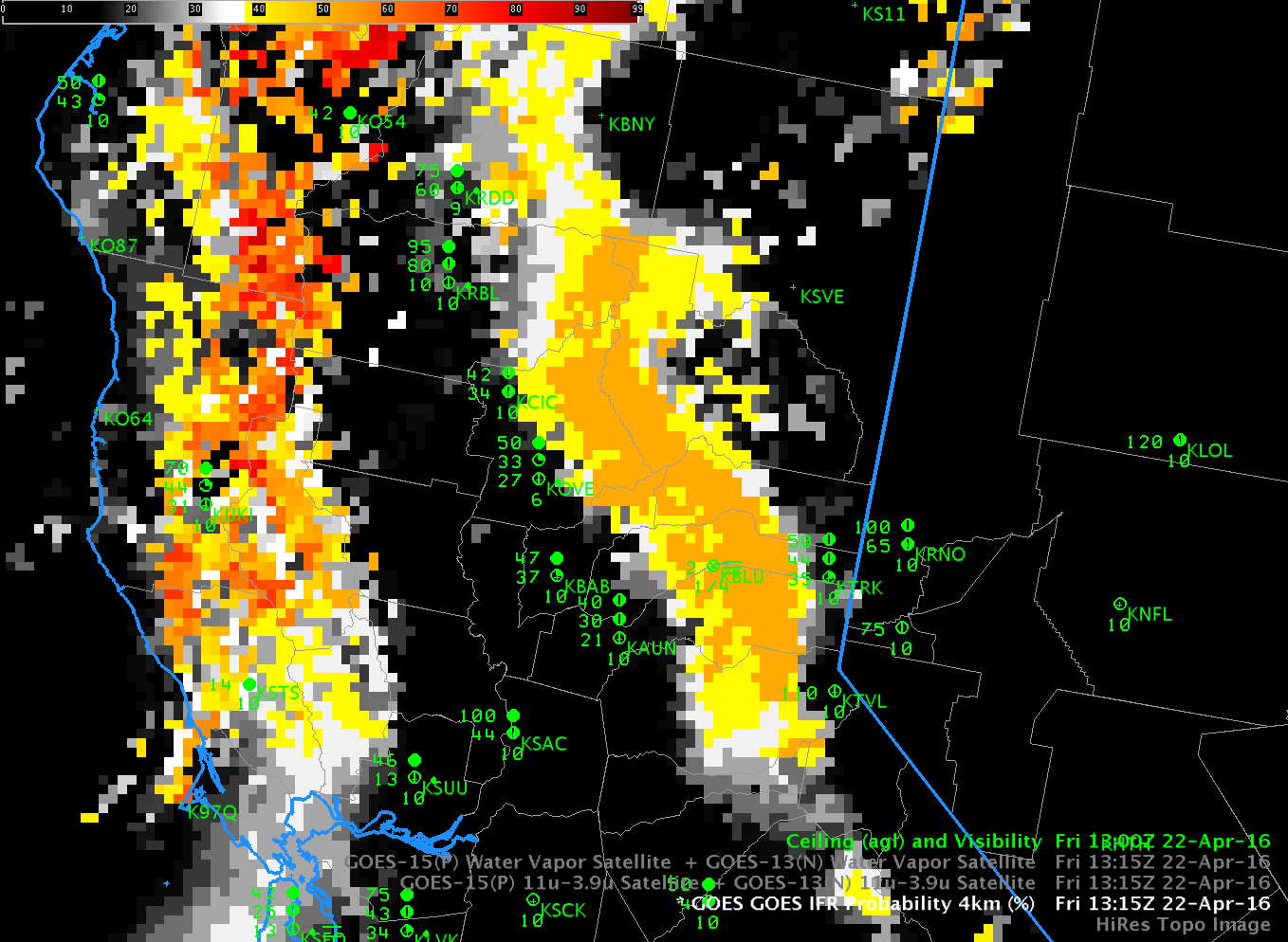
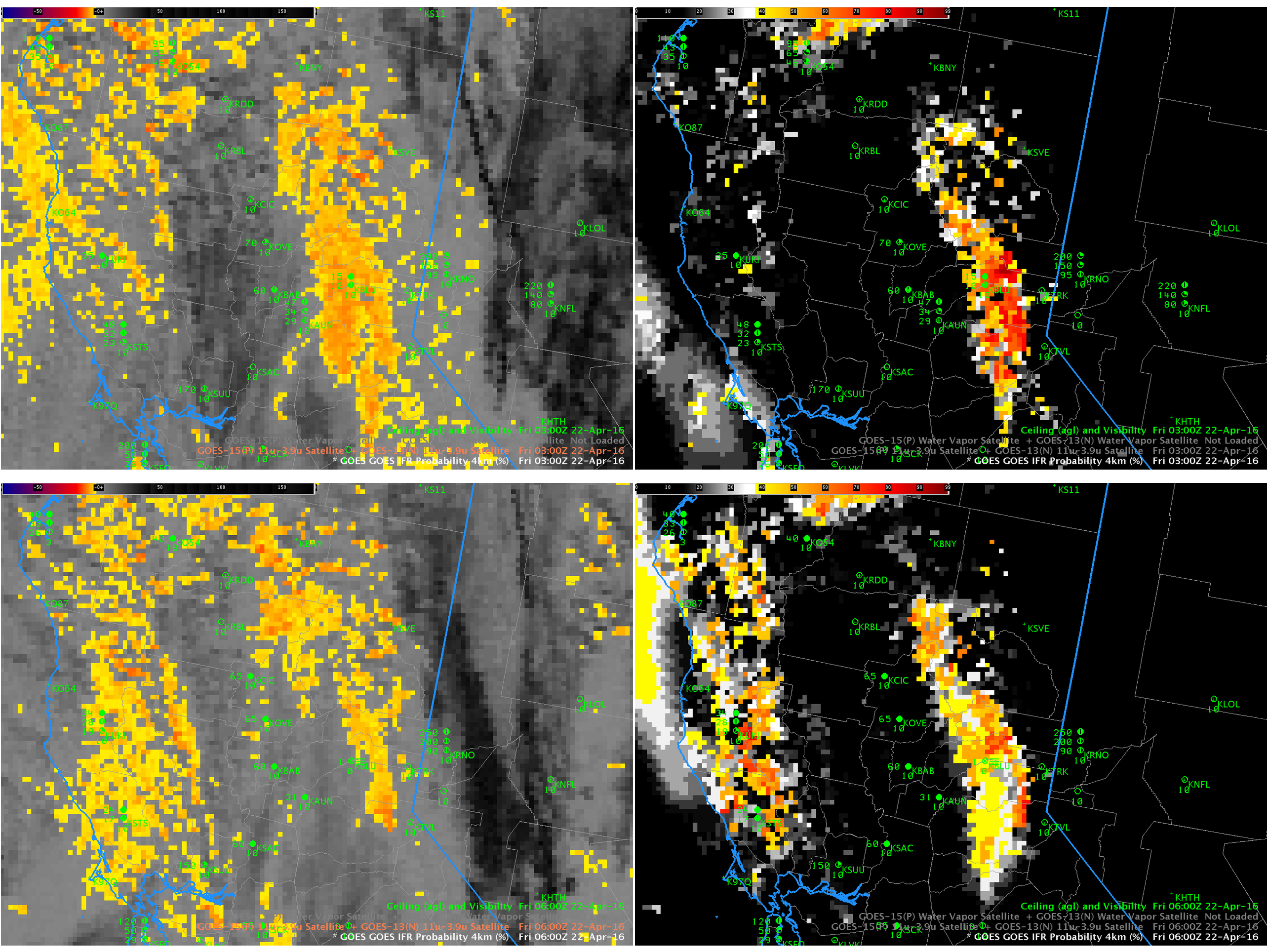
GOES-R IFR Probability fields on 27 June 2016 at 0200, 0400, and then hourly from 0700 through 1300 UTC (Click to enlarge)

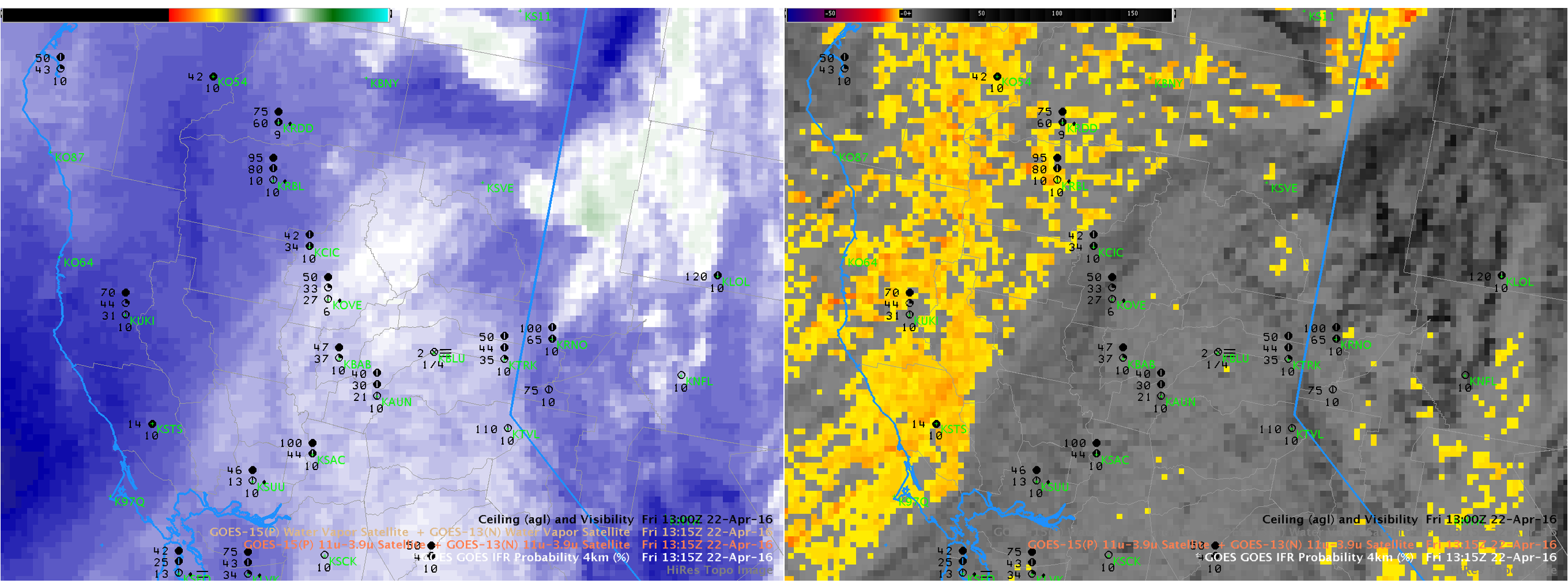
Late-day thunderstorms on 26 June 2016 set the scene for the development of fog overnight over southwestern Georgia. The animation above shows the GOES-R IFR Probability fields. An enhancement in the fields that is initially driven by Rapid Refresh Model data showing near-saturation at low levels is apparent at 0200 UTC. As clouds associated with the departing convection dissipate, satellite data could also be used as input into the IFR Probability fields. The toggle below of GOES-13 Brightness Temperature Difference fields (3.9 µm – 10.7 µm), at 0200 and 0400 UTC, shows the appearance of low-level clouds as mid-level and higher clouds (dark in the enhancement used) dissipate. By 0400 UTC, when satellite pixels finally start to suggest low clouds, fog had already started to develop. IFR Probability fields gave an early alert to the possibility of fog development on this day that was not possible from satellite data alone.

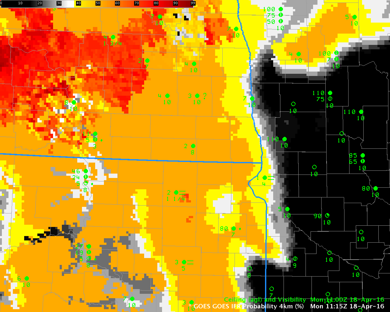
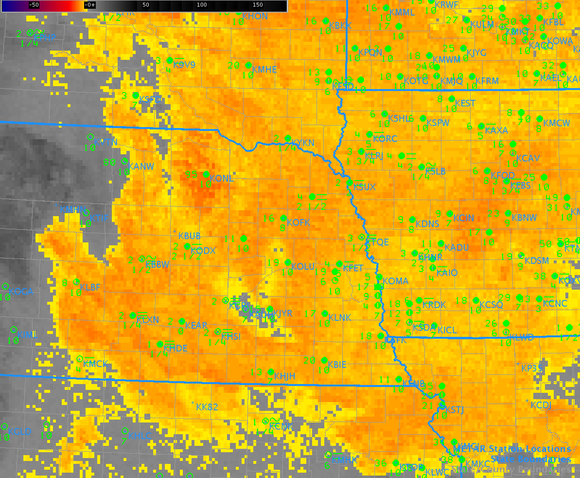
GOES-R Cloud Thickness Fields can give a hint to when radiation fog, as in this event, will dissipate in accordance with this scatterplot. The image below shows the GOES-R Cloud Thickness at 1030 UTC, the last field computed before twilight conditions (indeed, the boundary showing that boundary is readily apparent over eastern Georgia), with values exceeding 900 feet in some places over southwest Georgia. Based on the scatterplot, that suggests a dissipation time of just over 2 hours (based on the best fit line, but note the scatter in dissipation times associated with cloud thicknesses of 900 feet: just over an hour to almost 4 hours!) so clear skies would be expected by 1300 UTC. The animation of visible imagery, here, shows that fog persisted just a bit longer than that, dissipating shortly after 1400 UTC. GOES-R Cloud Thickness field is an empirical relationship between 3.9 µm emissivity and cloud thickness that is based on SODAR observations off the west coast. The scatterplot was created based on past observations limited to the southeast part of the US and parts of the Great Plains.

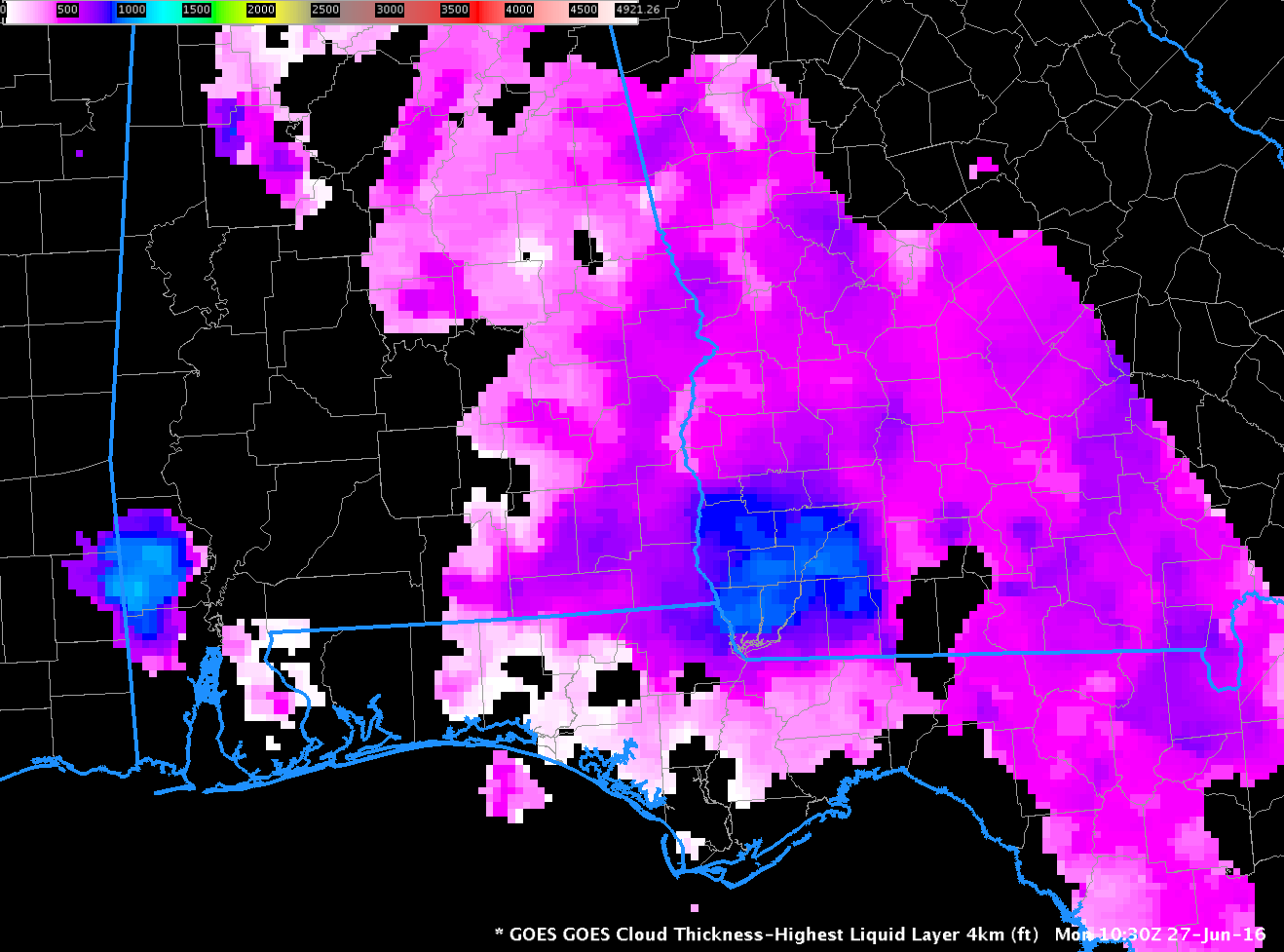
GOES-13 Cloud Thickness, 1030 UTC on 27 June 2016 (Click to enlarge)

Low Ceilings and reduced visibilities over the Ohio Valley

Surface Observations at 1200 UTC on 24 June 2016 (Click to enlarge)

A screen capture from this site at 1215 UTC on 24 June 2016, above, shows IFR Conditions (Red) and Low IFR Conditions (Purple) over the upper Ohio River Valley and surrounding states. The IFR Probability field for the same time, below, shows high probabilities in roughly the same regions that have IFR or Low IFR conditions. The Brightness Temperature Difference field, also displayed in the toggle below, gives little information at this time of day. A benefit of the GOES-R IFR Probability field is that it contains a coherent signal through sunrise.

GOES-R IFR Probability fields and GOES-13 Brightness Temperature Difference Fields (3.9 µm – 10.7 µm) at 1215 UTC on 24 June 2016 (Click to enlarge)

The toggle at 0915 UTC, below, before sunrise, shows a second benefit of IFR Probability fields: a useful signal in regions with cirrus clouds. High clouds, of course, prevent GOES-13 from viewing the development of fog/low stratus near the surface. The Rapid Refresh model data on low-level saturation that are part of the IFR Probability Field computations give quality information in regions of cirrus. In the example below, developing IFR conditions are depicted (the yellow enhancement that shows IFR Probabilities around 40%) over much of northern Kentucky and southern Ohio. This is under a region of cirrus (black in the enhancement used for the brightness temperature difference) north of a convective system that sits over southeastern Kentucky and eastern Tennessee.

GOES-R IFR Probability fields and GOES-13 Brightness Temperature Difference Fields (3.9 µm – 10.7 µm) at 0915 UTC on 24 June 2016 (Click to enlarge)

The waning full moon provided ample illumination for the Suomi NPP Day/Night Band Imagery, shown below, from 0736 UTC on 24 June 2016. The cirrus shield, mid-level clouds and developing valley fogs are all apparent.

Suomi NPP Day/Night band imagery, 0736 UTC on 24 June 2016 (Click to enlarge)

Multiple Cloud Layers and Topography

GOES-R IFR Probability Fields, 1315 UTC on 22 April 2016, along with surface observations of ceilings and visibilities (Click to enlarge)

The 1315 UTC image of GOES-R IFR Probabilities, above, shows an axis of higher probabilities aligned with the topography of the Sierra Nevada. Note that Blue Canyon (KBLU) is the sole station reporting IFR Conditions. Did conventional satellite data capture this event? The Water Vapor (6.5µm) and Brightness Temperature Difference fields (10.7µm – 3.9µm), below, do not show evidence of low clouds; indeed, the cirrus signature in the water vapor must mask any satellite observation of low clouds banked along the Sierra Nevada. Thus a fused product that combines model data and satellite data (such as IFR Probability fields) must be used, and the relatively flat nature of the IFR Probability field above confirms that Rapid Refresh information on low-level saturation is the reason why IFR Probability values are elevated along the mountains.

GOES-15 Water Vapor (6.5 µm), left, and GOES-15 Brightness Temperature Difference Field (10.7 µm – 3.9 µm), right, at 1315 UTC 22 April 2016 (Click to enlarge)

IFR Probability Fields earlier in the night did have a satellite component to them. The values at 0300 and 0600, below, show the gradual encroachment of cirrus from the south and west over the low clouds along the Sierra Nevada. After 0600 UTC, only model data were used over the Sierra as high-level cirrus blocked the satellite view.

Brightness Temperature Difference (10.7µm – 3.9µm) Fields (Left) and GOES-R IFR Probaility Fields (Right) from 0300 (Top) and 0600 (Bottom) on 22 April 2016 (Click to enlarge)

Reduced Visibilities under multiple cloud layers in the Northern Plains

GOES-R IFR Probabilities at 1115 UTC and 1100 UTC surface observations of ceiling and visibility (Click to enlarge)

The image above shows GOES-R IFR Probabilities over North/South Dakota and Minnesota shortly before sunrise on Monday April 18 2016. There is a distinct difference in the field between western Minnesota and eastern North and South Dakota that occurs because Rapid Refresh model fields (low-level saturation) are used as a predictor of IFR Probability. Reduced visibilities and ceilings are reported where IFR Probabilities exceed 50% (the orange shading). In contrast, the window channel and water vapor imagery for the same time, below, gives little indication that fog and low ceilings are present over eastern North and South Dakota: satellite views of the lowest levels are blocked by mid- and upper-level clouds. Fusing model data and satellite data into one predictor yields a superior product for detection of low ceilings and reduced visibilities.

GOES Infrared imagery (10.7 µm and 6.5 µm) and GOES-R IFR Probability fields, 1115 UTC on 18 April (Click to enlarge)

GOES-R IFR Probability screens out mid-level stratus

GOES-13 Brightness Temperature Difference (10.7 µm – 3.9 µm) at 1215 UTC on 29 March 2016 (Click to enlarge)

Consider the brightness temperature difference field above, from 1215 UTC on 29 March 2016. A strong signal that indicates water-based clouds extends from central Oklahoma to west Texas, and also from south Texas to west Texas. Are these water-based clouds obscuring visibilities at the surface? Over much of the region they are not. The Brightness Temperature Difference field gives information about the top of the cloud, but not the cloud base.

The GOES-R IFR Probability field for the same time, below, has screened out much of the region of mid-level stratus over Oklahoma and Texas. This can occur because IFR Probability fields include information from the Rapid Refresh Model. If that model does not indicated low-level saturation, IFR Probabilities will not be large. In the example shown, large values of IFR Probabilities are restricted to regions where IFR or near-IFR conditions are occurring.

GOES-R IFR Probability Fields at 1215 UTC on 29 March 2016 (Click to enlarge)

Widespread IFR conditions over the Upper Midwest

GOES-R IFR Probability Fields, hourly from 0215-1215, 14 March 2016 (Click to enlarge)

A rain-dampened boundary layer allowed fog to form over much of the upper midwest on early Monday March 14 2016 (as a baggy low pressure system moved eastward). GOES-R IFR Probability fields, above, captured the slow expansion of the region of IFR conditions. The character of the IFR Probability Field varies from smooth (over northern Illinois at 0215 UTC, for example (link)) to pixelated (over southern Minnesota at the same time). This is related to whether the model only is used as a predictor (over northern Illinois) because of high clouds that prevent the satellite from viewing low clouds or whether model and satellite data are both used as predictors (over southern Minnesota). The toggle below, of IFR Probability Fields and Brightness Temperature Difference fields at 1000 UTC on 14 March, underscores this relationship between IFR Probability and Brightness Temperature Difference fields.

In the animation above, IFR conditions are in general observed where IFR Probability fields suggest their presence.

GOES-R IFR Probability and GOES-13 Brightness Temperature Difference Field, 1000 UTC on 14 March 2016 (Click to enlarge)

Nebraska Fog

GOES-R IFR Probability fields, hourly from 0415 to 1515 UTC on 22 February, along with surface observations of ceilings and visibilities (Click to enlarge)

Dense Fog developed in two regions over Nebraska overnight, as shown in the screen capture below (from 1445 UTC) showing Dense Fog Advisories. GOES-R IFR Probabilities discerned the differences between the two regions, as shown in the animation above. The fog feature near the Missouri River (the boundary between Iowa and Nebraska) developed first in a region where high clouds were also present. That high clouds are present is apparent from the flat nature (that is, not pixelated) of the IFR Probability field at, say, 0415 and 0515 over western Iowa. The second region of fog, over south-central Nebraska, develops under clear skies as evidences by the (initially) very pixelated field. Towards the end of the animation high clouds overspread that region also. When that happens, IFR Probability values drop (because only model predictors can be used in the computation of IFR Probability in regions where high clouds exist). At the end of the animation, largest IFR Probabilities overlap the two regions where Dense Fog Advisories were issued. The region in between the advisories has lower Probabilities.

Compare the IFR Probability field, above, to Brightness Temperature Difference, below. Brightness Temperature Difference fields identify regions of Fog and Stratus, but near-surface information cannot be extrapolated (consistently) from cloud-top information. Thus, many stations with ceilings and visibilities far better than IFR conditions are in regions where a strong Brightness Temperature Difference signal exists (for example, KONL in northeastern Nebraska), The incorporation of surface information via Rapid Refresh model predictions of near-surface saturation allows the IFR Probability fields to better outline regions of IFR conditions only.

GOES-13 Brightness Temperature Difference (10.7 µm – 3.9 µm), 1300 UTC on 22 February 2016 (click to enlarge)

IFR Conditions with a Coastal Storm

GOES-R IFR Probabilities, hourly from 0400 through 1515 UTC, 5 February 2016 (Click to enlarge)

IFR Conditions frequently occur with storms along the East Coast. Satellite detection of such conditions is very difficult because of the multiple cloud layers that accompany cyclogenesis. The IFR Probabilities, above, have a character that reflects their determination solely from Rapid Refresh Data. That is, Satellite Predictors were not considered over much of New England because of the presence of multiple cloud layers, as suggested in the Water Vapor animation below.

IFR Probability fields are initially entirely offshore in the animation above, and IFR conditions are not observed over southern New England. Note how IFR probabilities initially increase over land over southern New Jersey and then quickly move northeastward into southern New England as IFR Conditions develop. Because satellite predictors are unavailable in these regions (on account of the many clouds layers), the simultaneous development of high IFR Probabilities with observed IFR Conditions argues for a good simulation of the observed weather by the Rapid Refresh. Fused data products such as IFR Probability fields join the strengths of different systems to provide a statistically more robust field than is possible from the individual pieces.

When daytime arrives — at around 1215 UTC in the animation above — a distinct transition is apparent in the GOES-R IFR Probability fields. This occurs because Satellite Data — visible satellite data — can be used during daytime to articulate the regions of cloudiness with more precision. Because cloudiness in general is better defined, IFR Probability fields (that require the presence of clouds) increase somewhat, and the color table used emphasizes that change.

GOES-13 Water Vapor 3-hourly Animation, 0400-1300 UTC, 5 February 2016 (Click to enlarge)

Near-IFR conditions over South Carolina

4Panel_IFR_BTD_CLDTHICK_WV_VIS_0300_1400anim

GOES-R IFR Probability (Upper Left), GOES-R Cloud Thickness (Lower Left), GOES-East Brightness Temperature Difference (10.7µm – 3.9µm) (Upper Right), GOES-East Water Vapor (6.5µm) at night, Visible Imagery (0.65µm) in day (Lower Right), hourly from 0315 UTC through 1400 UTC 29 January 2015 (Click to enlarge)

The animation above shows hourly imagery, from 0315 through 1400 UTC on 29 January 2016 (Click here for a faster animation). GOES-R IFR Probabilities are moving northeastward from South Carolina into North Carolina throughout the animation. Changes in surface observations of ceilings and visibilities closely match the motion of the GOES-R IFR Probability field. This is a case where the GOES-13 Brightness Temperature Field also is giving information about the presence of low clouds; GOES-R IFR Probability lends confidence to a forecaster that the stratus deck is actually fog because GOES-R IFR Probability includes information about low-level saturation (from the Rapid Refresh Model that is one of the predictors used in the statistical model used to generate IFR Probability fields).

In the early part of the animation, higher clouds are present and can be detected both in the water vapor imagery and in the brightness temperature difference (high clouds are dark in the enhancement curve used). When high clouds are present, GOES-R Cloud Thickness (in the lower left of the figures above) will not be determined as it is derived from an empirical relationship between the 3.9 emissivity of low clouds and cloud thickness that was determined from sodar observations of cloud thickness off the West Coast of the USA. High clouds prevent a determination of this relationship. Regions where GOES-R Cloud Thickness is not computed at night because of high clouds correspond very well with regions where GOES-R IFR Probability is determined by Rapid Refresh Model Output only.

Dense Fog and Freezing Fog in Montana and North Dakota

GOES-R IFR Probability Fields, 0300-1300 UTC on 20 January 2015 (Click to enlarge)

Dense Fog over North Dakota and Freezing Fog over eastern Montana prompted the issuance of Dense and Freezing Fog advisories early Wednesday Morning. GOES-R IFR Probabilities, above, computed from data from the GOES-13 Imager and from Rapid Refresh Model output, capture the growth/evolution of the fog field. In general, the IFR Probability field captures the area of reduced visibilities (with some exceptions, such as KHEI (Hettinger, ND, near the border with South Dakota is southwest North Dakota).

Compare the areal extent of the IFR Probability field with that from the Brightness Temperature Difference from GOES, below. The presence of multiple cloud layers prevents any satellite from viewing low clouds, and satellite-only products therefore give little information about near-surface events in much of western North Dakota and Montana. When Rapid Refresh Model output is controlling the GOES-R IFR Probability field, as happened in this case over Montana and western North Dakota, the IFR Probability will have lower values and a less pixelated look that reflects the coarser model resolution and model smoothing.

GOES Brightness Temperature Difference fields, 0300-1300 UTC, 20 January 2016 (Click to enlarge)

GOES-R Fog Product Examples

Fog detection fusing GOES, Terra/Aqua or Suomi/NPP Satellite data with Model output