Category Archives: Multiple Cloud Layers

Dense Fog under high clouds in the Deep South

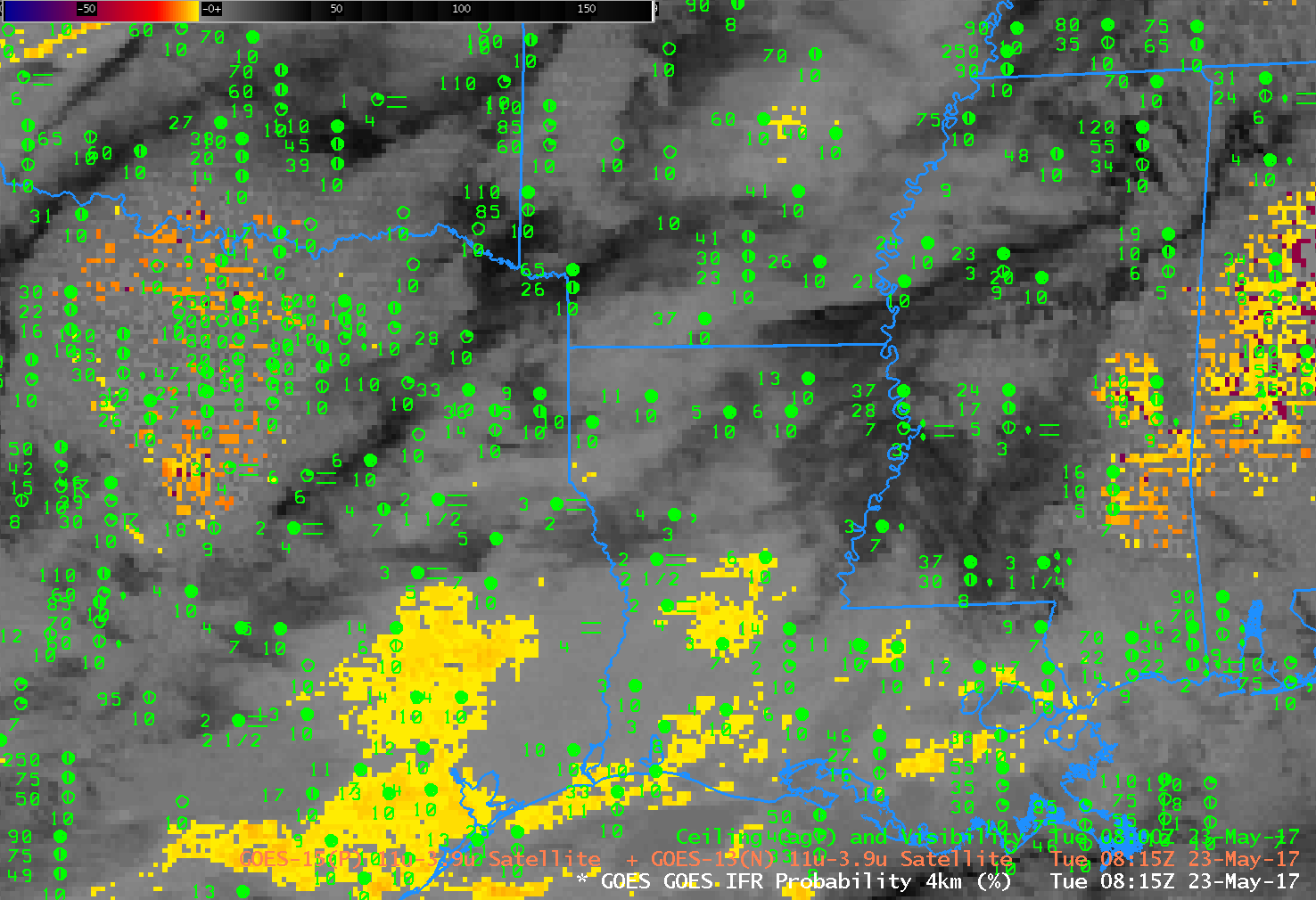
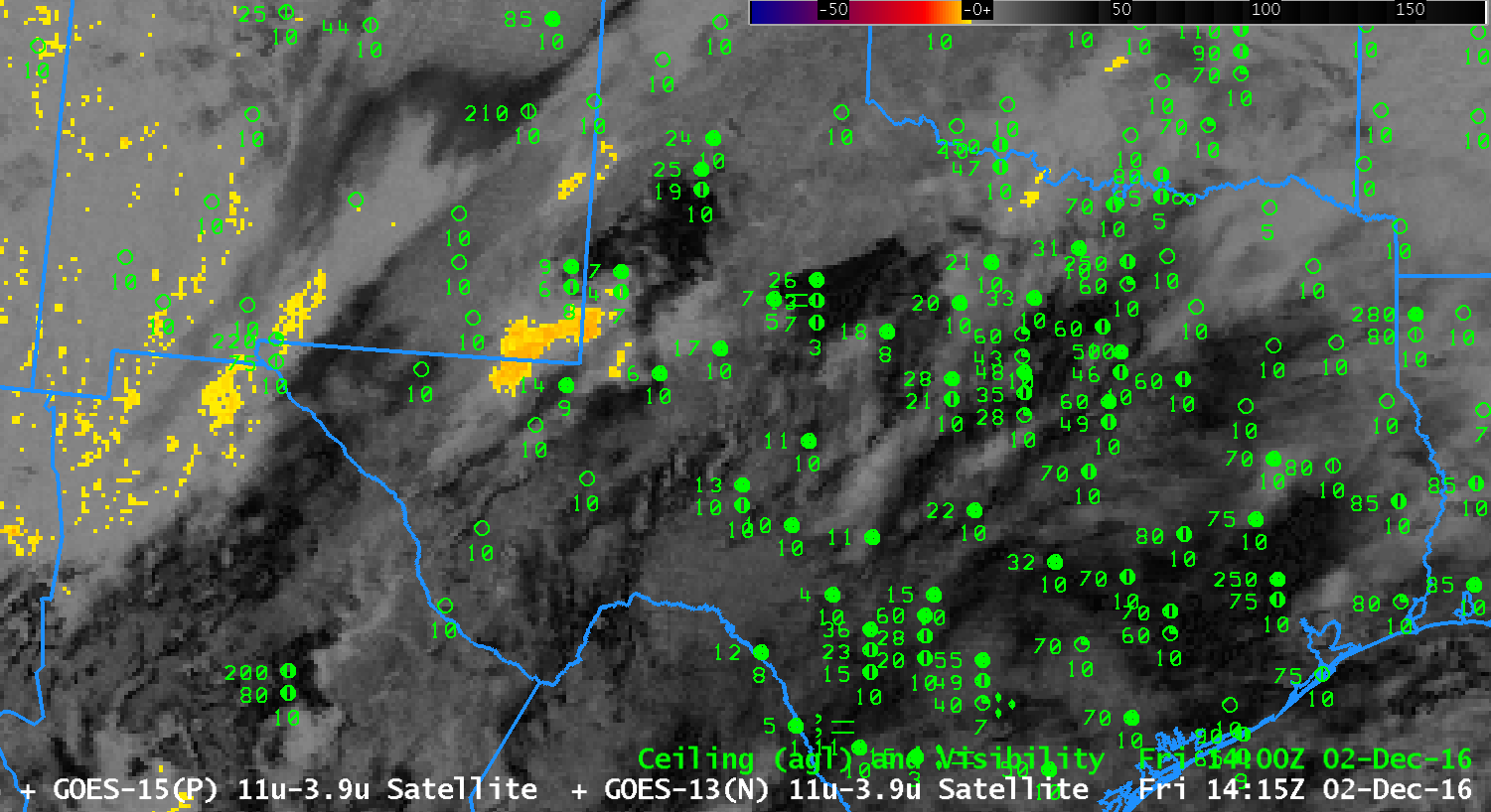
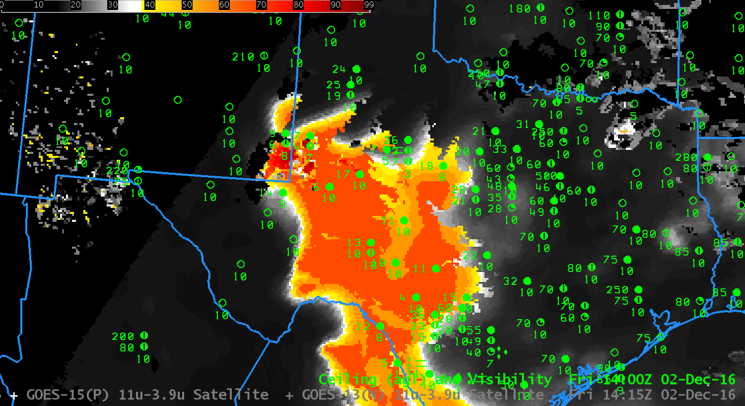
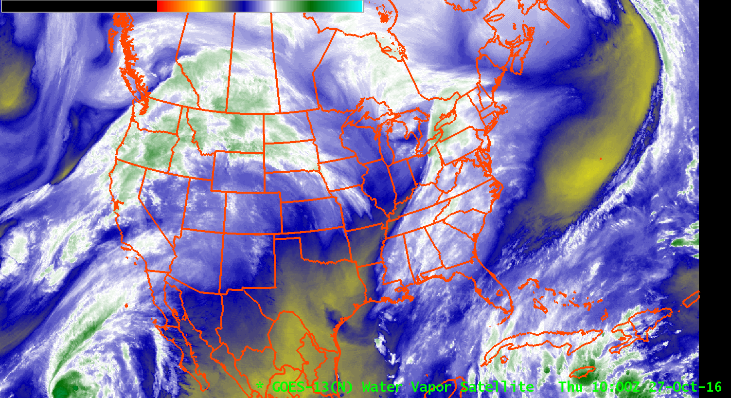
GOES-13 Brightness Temperature Difference (3.9 µm – 10.7 µm) Values at 0815 UTC on 23 May 2017 (Click to enlarge)

Note: GOES-R IFR Probabilities are computed using Legacy GOES (GOES-13 and GOES-15) and Rapid Refresh model information; GOES-16 data will be incorporated into the IFR Probability algorithm in late 2017

The legacy method of detecting fog/low clouds from satellite is the Brightness Temperature Difference product that compares computed brightness temperatures at 3.9 µm and at 10.7 µm. At night, because clouds composed of water droplets do not emit 3.9 µm radiation as a blackbody, the inferred 3.9 µm brightness temperature is colder than the brightness temperature computed using 10.7 µm radiation. In the image above, the brightness temperature difference has been color-enhanced so that clouds composed of water droplets are orange — this region is mostly confined to southeast Texas. Widespread cirrus and mid-level clouds are blocking the satellite view of low clouds. IFR and near-IFR conditions are widespread over east Texas, Louisiana and Mississippi. The GOES-R IFR Probability field, below, from the same time, suggests IFR conditions are likely over the region where IFR conditions are observed.

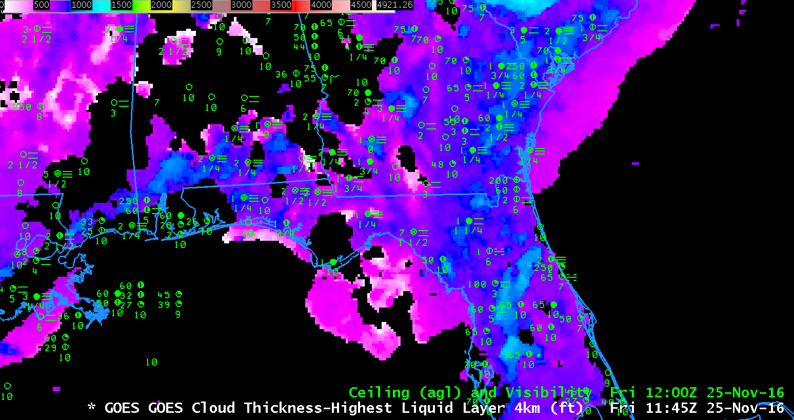
This is a case where the model information that is included in this fused product (that includes both satellite observations where possible and model predictions) fills in regions where cirrus and mid-level clouds obstruct the satellite’s view of low clouds.. As a situational awareness tool, GOES-R IFR Probability can give a more informed representation of where restricted visibilities and ceilings might be occurring.

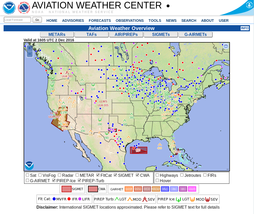
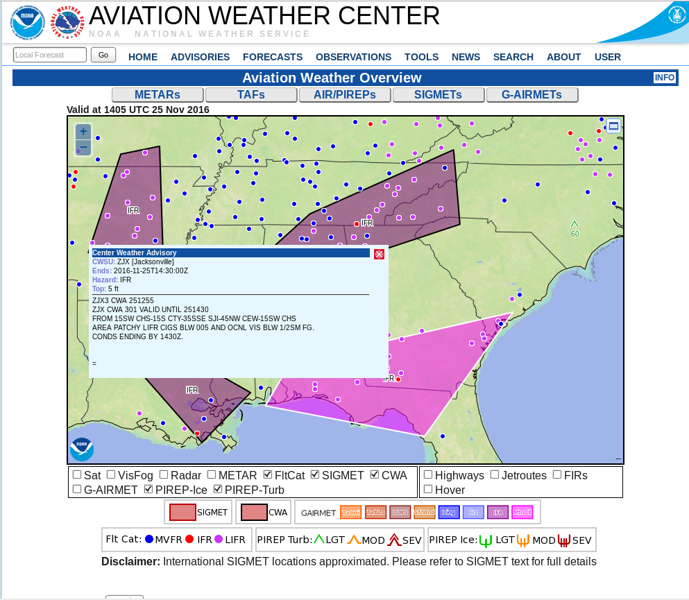
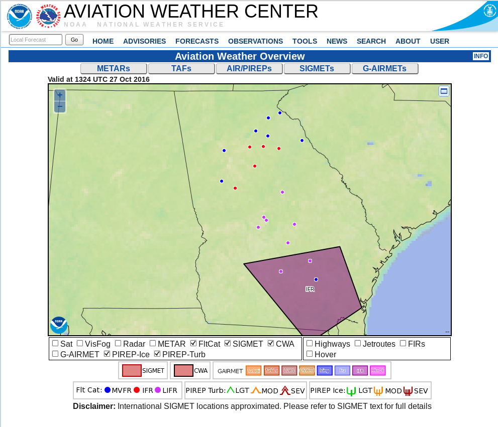
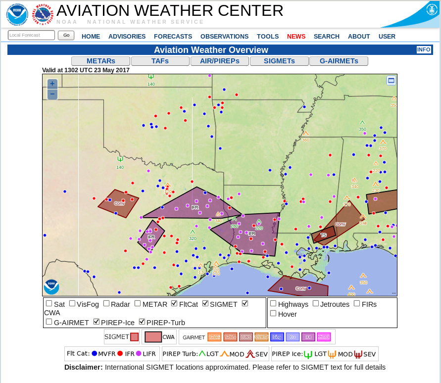
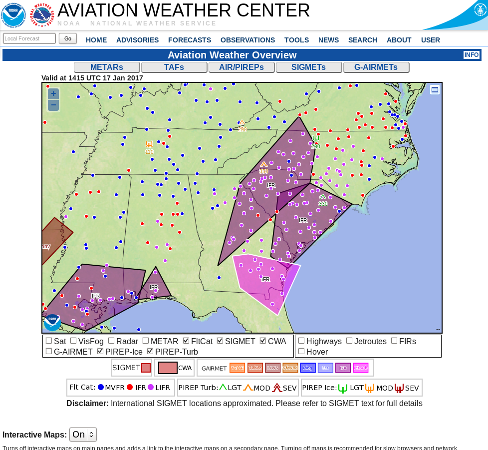
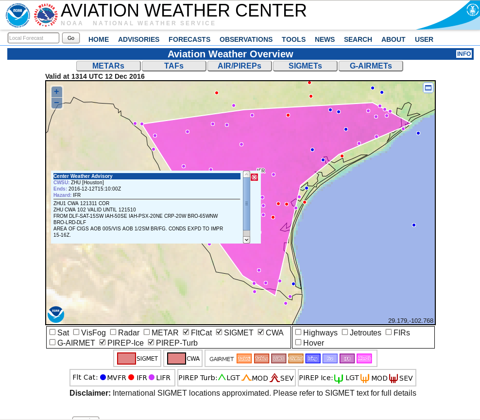
IFR Conditions continued into early morning as noted in this screenshot from the Aviation Weather Center.

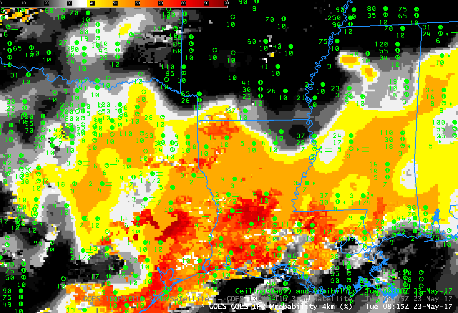
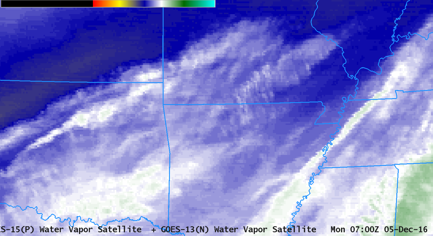
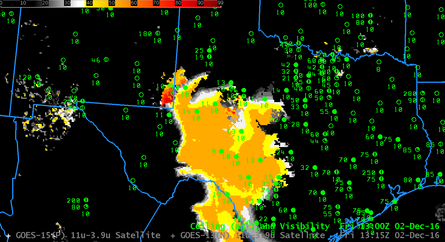
GOES-R IFR Probability fields, 0815 UTC on 23 May 2017 (Click to enlarge)

IFR Conditions under multiple cloud decks in the Upper Midwest

GOES-R IFR Probability Field, along with observations of surface visibility and ceiling heights, 1100 UTC on 17 May 2017 (Click to enlarge)

The GOES-16 data posted on this page are preliminary, non-operational data and are undergoing testing

A morning screenshot from the Aviation Weather Center website shows a wide region of IFR and Low IFR Conditions reported over the Upper Midwest, from eastern North Dakota eastward to Lake Superior. The GOES-R IFR Probability field, above, from 1100 UTC on 17 May 2017, shows high probabilities over that region.

Over much of Minnesota and Michigan, the character of the IFR Probability field is flat. This is typical of IFR Probability when high clouds prevent satellite data from being used as a statistical predictor for IFR Conditions. If high clouds are present, the satellite cannot detect the presence of low clouds, and the chief predictor of IFR conditions will therefore be model data that typically does not vary strongly from gridpoint to gridpoint when IFR conditions are present. The pronounced boundary apparent in the IFR Probability field that extends nortwestward from Green Bay in Wisconsin is the boundary between night-time predictors (to the west) and daytime predictors (to the east).

GOES-R IFR Probability values are largest in the region of IFR conditions over North Dakota. In this region, high clouds are not present and the satellite is able to detect low clouds, and that information is part of the computation of IFR Probabilities. Note also the region in east-central Minnesota where satellite data are also being used in the computation of IFR Probabilities; the resultant field there is pixelated.

The toggle below shows the brightness temperature difference field between the shortwave and longwave infrared window channels from GOES-13 (3.9 µm and 10.7 µm) and GOES-16 (3.9 µm and 10.33 µm). This brightness temperature difference field is used to detect stratus, and by inference fog, because stratus cloud tops composed of water droplets emit radiation around 10.3-10.7 µm as a blackbody, but do not emit 3.9 µm radiation as a blackbody. Satellite detection of radiation, and computation of the inferred temperature of the emitting surface, assumes blackbody emissions. Consequently, the brightness temperature computed using detected 3.9 µm radiation is colder than that computed using 10.7 µm (or 10.33 µm) radiation.

Both satellites capture the region of low stratus/fog over North Dakota, and the superior spatial resolution of GOES-16 is apparent. Note, however, that neither satellite can detect low clouds associated with dense fog in regions of higher clouds — over Michigan’s Keewenaw Peninsula, for example, or along the shore of Lake Superior in Minnesota. This is an unavoidable shortcoming of satellite-only-based detection of low clouds/fog.

GOES-13 (3.9 µm – 10.7 µm) and GOES-16 (10.33 µm – 3.9 µm) Brightness Temperature Difference fields, 1100 UTC on 17 May 2017 (Click to enlarge)

IFR Probabilities with a strong storm in Maine

GOES-R IFR Probabilities, 0100-1000 UTC on 7 April 2017, along with surface reports of ceilings and visibilities (Click to enlarge)

A strong storm over the northeastern United States produced widespread IFR conditions over that region. The storm was also accompanied by multiple cloud layers, however, and that made diagnosis of regions low clouds/fog difficult. For these cases, a fused data approach is vital — using model information (in the case of IFR Probability, above, the model is the Rapid Refresh) to provide information at low levels allows for a better tool to alert a forecaster to the presence of reduced visibilities.

In the animation above, Maine intially shows IFR Probabilities around 50% — but the flat nature of the field should alert a user to the fact that satellite predictors cannot be included in the computation of IFR Probabilities because high clouds are preventing a satellite view of low clouds. Accordingly, the computed Probability is lower. In contrast, high clouds are not present over southern New England at the start of the animation, and IFR Probabilities are much larger there: both satellite and model predictors are used. As the high clouds lift north from northern New England the region of higher IFR Probabilities expands from the south.

Note the influence of topographic features on the IFR Probability field. The Adirondack Mountains and St. Lawrence Seaway have higher and lower Probabilities, respectively, because of the higher terrain in the Mountains, and the lower terrain along the St. Lawrence.

An example of why fused data are important is shown below. Look at the conditions in Charlottetown, on Prince Edward Island, in the far northeast part of the domain. Between 0315 and 0400, ceilings and visibilities deteriorate as IFR Probabilities increase. The brightness temperature difference field, at bottom, shows no distinct difference between those two times because the clouds being viewed are high clouds.

Dense Fog over the Carolinas

GOES-13 Brightness Temperature Difference (3.9 µm – 10.7 µm), GOES-R IFR Probability and GOES-R Cloud Thickness at 1115 UTC on 17 January 2017 (Click the enlarge)

Dense Fog Advisories (National Weather Service Website) and IFR SIGMETs (Aviation Weather website) were issued early in the morning for dense fog over the southeastern United States. The toggle above from 1115 UTC on 17 January shows the Brightness Temperature Difference field (3.9 µm – 10.7 µm), the GOES-R IFR Probability Field, and the GOES-R Cloud Thickness fields associated with this dense fog event. Note the presence of high clouds over northern South Carolina and western North Carolina — the dark region in the Brightness Temperature Difference enhancement — prevents the brightness temperature difference field from highlighting that region of reduced ceilings/visibilities. The GOES-R Cloud Thickness field is not computed under cirrus either, as it relates 3.9 µm emissivity of water-based clouds to cloud thickness (based on a look-up table generated using data from a SODAR off the West Coast of the United States). If cirrus blocks the view, then, neither the Brightness Temperature Difference field nor the GOES-R Cloud Thickness field can give useful information about low clouds.

In contrast, the GOES-R IFR Probability field does give useful information in regions where cirrus clouds (and low clouds/fog) are present — because Rapid Refresh information about the lower troposphere can be used. IFR Probability values will be smaller in those regions because satellite predictors are unavailable, and the Probability incorporates both predictors from satellites and from Rapid Refresh model output — if the satellite predictors are missing because of cirrus, the IFR Probability values will be affected. Despite the smaller values, however, the IFR Probability fields in regions of cirrus are giving useful information for this event.

GOES-R Cloud thickness fields can be used to estimate Fog dissipation using the last GOES-R Cloud Thickness field produced before twilight conditions at sunrise (shown below for this case). (GOES-R Cloud Thickness is not computed during twilight conditions because of rapidly changing 3.9 µm emissivity related to the reflected solar radiation as the sun rises, or as it sets). This scatterplot gives the relationship between thickness and dissipation time after the Cloud Thickness time stamp (1215 UTC in this case). In this case, the thickest fog is near Athens GA; the algorithm predicts that clearing should happen there last, at about 1515 UTC.

GOES-R Cloud Thickness, 1215 UTC on 17 January 2017 (Click to enlarge)

Fog over South Texas

Toggle between Brightness Temperature Difference (3.9µm – 10.7µm) and GOES-R IFR Probability fields, 2300 UTC on 11 December 2016 (Click to enlarge)

Dense Fog developed over south Texas during the early morning of 12 December 2016 (IFR Sigmet from this website shown here ; Advisories from the weather.gov website shown here). The toggle above shows in the brightness temperature difference field a signature of high clouds — and where those high clouds exist, IFR Probability fields rely on Rapid Refresh Model data to diagnose where IFR conditions might be occurring, or where IFR conditions might develop. The animation of Brightness Temperature Difference fields from 0215 through 1115 UTC, below, shows that the high clouds over south Texas diminished with time: by 0815 UTC only low stratus is present over south Texas. But is that stratus also hugging the ground — that is, is it fog? From the satellite’s perspective, the top of a stratus deck and the top of a fog bank can look very similar.

GOES-13 Brightness Temperature Difference (3.9µm – 10.7µm), 0215 through 1115 UTC on 12 December (Click to enlarge)

GOES-R IFR Probability fields give a more complete estimate about the presence of fog/low stratus because Rapid Refresh data and satellite data are used to diagnose the probability of IFR conditions. If the Rapid Refresh model shows low-level saturation, then the presence of stratus clouds also likely indicates the presence of fog; conversely, if the Rapid Refresh Model does not show low-level saturation, then the presence of stratus cloud need not indicate the presence of fog. IFR Probability fields below, from 0215 through 1115 UTC, start off regions with uniform values where only Rapid Refresh data are used in the algorithm — where high clouds block the satellite view of low clouds/fog. As the high clouds dissipate, the field acquires larger values because there is higher confidence of the presence of clouds (in part because satellite data can be used to observe them). In addition, these larger values have pixel-sized variability because of variability in the satellite observations.

IFR conditions are observed latest over far south Texas — this is also where IFR Probabilities are slowest to reach large values.

Fog and Ice Fog over the southern Plains

GOES-R IFR Probabilities, hourly from 0400 through 1215 UTC on 5 December 2016 (Click to enlarge)

Dense Fog developed over the southern Plains early on Monday 5 December, and the GOES-R IFR Probability fields, above, were a tool that could be used to monitor the evolution of this event. A challenge presented on this date was the widespread cirrus (Here’s the 0700 UTC GOES-13 Water Vapor (6.5 µm) Image, for example) that prevented satellite detection of low clouds. The Brightness Temperature Difference fields, below, at 3-hourly intervals, also show a signature (dark grey/black in the enhancement used) of high clouds, although they are shifting east with time — by 1300 UTC there is a signature (orange/yellow in the enhancement used) of stratus clouds over central and eastern Oklahoma.

The IFR Probability fields, above, have a characteristic flat nature over Arkansas and Missouri, that is, a uniformity to the field, that is typical when model data are driving the probabilities. The more pixelated nature to the fields over Kansas and Oklahoma, especially near the end of the animation, typifies what the fields look like when both satellite data and model data are driving the computation of probabilities. Careful inspection of the fields over Arkansas shows regions — around Fayetteville, for example, around 1000 UTC where IFR Probabilities are too low given the observation at the airport of IFR conditions. This inconsistency gives information on either the small-scale nature of the fog (unlikely in this case) or on the accuracy of the Rapid Refresh model simulation that is contributing to the probabilities. In general, the Rapid Refresh model has accurately captured this event, and therefore the IFR Probabilities are mostly overlapping regions of IFR or near-IFR conditions. The region over southern Illinois that has stratus, and low probabilities of IFR conditions, for example. Adjacent regions have higher IFR Probabilities and lower ceilings and/or reduced visibilities. A screen shot from the National Weather Service, and from the Aviation Weather Center, at about 1300 UTC document the advisories that were issued for this event.

Brightness Temperature Difference fields (3.9 µm – 10.7 µm), 0400, 0700, 1000 and 1300 UTC on 5 December 2016 (Click to enlarge)

IFR Conditions over the High Plains of west Texas

GOES-13 Brightness Temperature Difference (3.9 µm – 10.7 µm, left) and GOES-R IFR Probability Fields (Right), hourly from 0215 through 1415 UTC on 2 December 2016 (Click to enlarge)

Near-IFR and and IFR Conditions developed over the High Plains of Texas on 2 December 2016, and a SIGMET for IFR conditions was issued as shown below.

The animation above shows plentiful cirrus (in the brightness temperature difference enhancement used in the imagery on the left, above, cirrus clouds are dark) over south Texas, with occasional breaks. This makes continual monitoring via satellite of the developing stratus/fog field problematic: the satellite cannot monitor what it is blocked from being observed by intervening cloud layers — in this case cirrus. (Click here for a brightness temperature difference only animation; Click here for an IFR Probability only animation) Because IFR Probability fields include model-based data about saturation in the lower troposphere, in the form of Rapid Refresh model output, a useful and coherent signal can be generated underneath cirrus clouds. The GOES-R IFR Probability signal can be better used for situational awareness and anticipation of the development of the IFR conditions shown below.

In the animation above, note the change between 1315 and 1415 UTC fields — in the Brightness Temperature Difference fields (1315 UTC ; 1415 UTC), this change arises because of increasing amounts of reflected solar 3.9 µm radiation: this causes a sign change in the brightness temperature difference. For IFR Probability fields (1315 UTC ; 1415 UTC), the change occurs because the Predictors used at night (1315 UTC) and during the day (1415 UTC) are different.

1605 UTC screen capture from Aviation Weather Center. Note IFR Sigmet over west Texas (Click to enlarge)

Dense Fog in Georgia and Florida

GOES-R IFR Probability Fields, 0000 – 1300 UTC on 25 November 2016 (Click to enlarge)

Light winds and a long November night allowed radiation fog formation over much of the deep south early on 25 November 2016. (1200 UTC Surface analysis is here). The Aviation Weather Center Website indicated widespread IFR Conditions, below, over the south, with the sigmet suggesting improving visibilities after 1400 UTC.

The animation above shows the evolution of the GOES-R IFR Probability fields from just after sunset to just after sunrise. There is a good spatial match between observed IFR conditions and the developing field. IFR Probability can thus be a good situational awareness tool, identifying regions where IFR Conditions exist, or may be developing presently.

Screenshot of Aviation Weather Center Front Page, 1405 UTC on 25 November (Click to enlarge)

Did the GOES-13 Brightness Temperature Difference Field identify the fields? The animation below, from 0200-1300 UTC, shows a widespread signal that shows no distinguishable correlation with observed IFR conditions. Note also how the rising sun at the end of the animation changes the difference field as more and more reflected solar radiation with a wavelength of 3.9 µm is present. In addition, high clouds that move from the west (starting at 0400 UTC over Louisiana) prevent the satellite from viewing low clouds in regions where IFR conditions exist.

GOES-13 Brightness Temperature Difference field (3.9 µm – 10.7 µm), 0200-1300 UTC on 25 November 2016 (Click to enlarge)

The high clouds that prevent satellite detection of low clouds, as for example at 1100 UTC over parts of Alabama, cause a noticeable change in the IFR Probability fields, as shown in the toggle below. Values over the central part of the Florida panhandle are suppressed, and the field itself has a flatter character (compared to the pixelated field over southern Georgia, for example, where high clouds are not present). Even though high clouds prevent the satellite from providing useful information about low clouds in that region, GOES-R IFR Probability fields can provide useful information because of the fused nature of the product: Rapid Refresh information adds information about low-level saturation there, so IFR Probability values are large. In contrast, over southern Florida — near Tampa, for example, Rapid Refresh data does not show saturation, and IFR Probabiities are minimized even through the satellite data has a strong signal — caused by mid-level stratus. Soundings from Tampa and from Cape Kennedy suggest the saturated layer is around 800 mb.

GOES-R IFR Probability fields and GOES-13 Brightness Temperature Difference Fields, 1100 UTC on 25 November 2016 (Click to enlarge)

GOES-R Cloud Thickness, below, related 3.9 µm emissivity to cloud thickness via a look-up table that was generated using GOES-West Observations of marine stratus and sodar observations of cloud thickness. The last pre-sunrise thickness field, below, is related to dissipation time via this scatterplot. The largest values in the scene below are around 1000 feet, which value suggests a dissipation time of about 3 hours, or at 1445 UTC.

GOES-R Cloud Thickness Field, 1145 UTC on 25 November 2016 (Click to enlarge)

IFR Probability Fields let you peek beneath the Cirrus

GOES-13 Brightness Temperature Difference (3.9 µm – 10.7 µm) fields, hourly from 0215-1215 UTC on 27 October (Click to enlarge)

If you rely on satellite data alone to anticipate the development of IFR conditions — fog, low ceilings, and reduced visibilities — then the presence of widespread cirrus, shown here with the GOES-13 6.5 µm image, makes situational awareness difficult. At a glance, can you tell in the animation of brightness temperature difference, above, hourly from 0215 through 1215 UTC, where IFR Conditions are occurring? The widespread cirrus, present in the enhancement as dark grey and black, prevents the satellite from viewing any fog development, hence making this brightness temperature difference field, traditionally used to detect the development of fog and low stratus, unsuitable for large-scale situational awareness.

GOES-R IFR Probability fuses satellite data with Rapid Refresh Model output and allows a product that in essence peeks beneath the cirrus because near-surface saturation predicted in the Rapid Refresh Model allows the IFR Probability product to have a strong signal where fog might be developing. Consider the animation below, that covers the same spatial and temporal domain as the brightness temperature difference animation above. IFR Probability increases over inland southeast Georgia in concert with the development of low ceilings/reduced visibilities. It gave a few hours alert to the possibility that IFR conditions would be developing. Note in the animation below that the 1215 UTC image includes IFR Probabilities computed using daytime predictors and nighttime predictors. There is therefore a discontinuity in the field values over central Georgia at 1215 UTC, the end of the animation.

Compare the animation below to the one above. Which yields better situational awareness for the developing fog field?

GOES-R IFR Probability Fields, hourly from 0215 through 1215 UTC on 27 October (Click to enlarge)

The Aviation Weather Center plot (below) highlights the presence of an IFR SIGMET over the region at 1324 UTC on 27 October.

Aviation Weather Center plot showing MVFR, IFR and LIFR stations over Georgia, along with an IFR Sigmet at 1324 UTC 27 October 2016 (Click to enlarge)

IFR Probability Screens out mid-level Stratus

GOES-13 Brightness Temperature Difference (3.9 µm- 10.7 µm) and GOES-R IFR Probability fields computed with GOES-13 and Rapid Refresh Data, 1100 UTC 18 October. Plots of ceilings and surface visibilities are included (Click to enlarge)

GOES-R IFR Probability fields often to a better job (compared to brightness temperature difference fields) in outlining exactly where low ceilings and reduced visibilities are occurring because IFR Probability fields include information about low-level saturation from the Rapid Refresh model. That information about near-surface saturation allows the IFR Probability algorithms to screen out regions where only mid-level stratus is occurring. A low fog — a stratiform cloud of water droplets that sits on/near the surface — and a mid-level stratus deck (also a stratiform cloud of water droplets) can look very similar in a brightness temperature difference field. In the example above, consider much of northeastern Alabama and northern Georgia. There is a strong return in the brightness temperature difference field because mid-level stratus is present — but IFR Probabilities are small because the Rapid Refresh does not diagnose low-level saturation in the region. Compare Brightness Temperature Difference returns over northeast Alabama and over extreme western North Carolina — to the west of Asheville. IFR Conditions are observed over western North Carolina, and IFR Probabilities are high there. In general, the region with high IFR Probabilities in the toggle above includes stations that are reporting IFR or near-IFR conditions. Most stations outside the region of high IFR Probability are not showing IFR Conditions, even though they may be in a region with the Brightness Temperature Difference signal is large.

A similar story can be told farther west at 0800 UTC, shown below. Focus on the region with a strong Brightness Temperature Difference signal over southeast Arkansas. IFR Conditions are not occurring under that mid-level stratus deck, and IFR Probabilities are very low. Similarly, IFR Probabilities are small over Oklahoma and north-central Texas because the Rapid Refresh Model is not showing low-level saturation in those regions; IFR Probabilities cannot be large when low-level saturation is not indicated in the model.

Using both Satellite Data and Model Data accentuates the strengths of both. That’s the power of a fused data product.

GOES-13 Brightness Temperature Difference (3.9 µm – 10.7 µm) and GOES-R IFR Probability fields computed with GOES-13 and Rapid Refresh Data, 0800 UTC 18 October. Plots of ceilings and surface visibilities are included (Click to enlarge)

GOES-R Fog Product Examples

Fog detection fusing GOES, Terra/Aqua or Suomi/NPP Satellite data with Model output