Category Archives: MODIS

Fog and Stratus under high clouds in the Southern Plains

GOES-13-based GOES-R IFR Probabilities (Upper Left), GOES-13 Brightness Temperature Difference Product (10.7 µm – 3.9 µm) (Upper Right), MODIS-based GOES-R IFR Probabilities (Lower Left), Suomi-NPP Brightness Temperature Difference (11.35 µm – 3.74 µm) and Day/Night band (Lower Right), all times as indicated (click image to enlarge)

Fog and low stratus developed over the Southern Plains during the morning hours of 28 October 2013. The imagery above, from near 0730 UTC, demonstrates strengths of the IFR Probability fields and inherent limitations to the traditional methods of detecting fog and low stratus: the brightness temperature difference between 10.7 µm and 3.9 µm data. For example, note the elevated stratus over the Red River Valley in southeastern OK. Both GOES and VIIRS Brightness Temperature Difference fields there show a strong signal (and the day/night band also suggest clouds are present); IFR Probabilities are low, however, and are in good agreement with the observed ceilings and visibilities that show MVFR conditions.

The brightness temperature difference fields from both Suomi/NPP and from GOES show high clouds over south-central OK, in a region where IFR Conditions are observed. Rapid Refresh model data are being used in this region to diagnose — accurately — the presence of visibility-restricting fog and low stratus. As is typical when Rapid Refresh data are the primary means of diagnosing IFR Probabilities (because high clouds prevent the satellite from seeing water-based clouds near the surface), the IFR probability field is smooth.

IFR Conditions in the northern Plains

GOES-13-based GOES-R IFR Probabilities (Upper Left), GOES-13 Brightness Temperature Difference Product (10.7 µm – 3.9 µm) (Upper Right), MODIS-based GOES-R IFR Probabilities (Lower Left), Suomi-NPP Brightness Temperature Difference (11.35 µm – 3.74 µm) (Lower Right), all times as indicated (click image to enlarge)

The animation above shows GOES-R IFR Probabilities highest in a band that stretches mostly north-south from western North Dakota into central South Dakota. IFR conditions are observed under and near this band, for example at Stanley, North Dakota. The occasional MODIS-based IFR Probabilities also suggest that IFR conditions are most likely over the western Dakotas. Both GOES-based and MODIS-based IFR Probability fields de-emphasize the regions of enhanced brightness temperature difference (in both GOES and Suomi-NPP Fields) that exist over western Minnesota and the central and eastern Dakotas. In these regions, mid-level stratus is being detected by the satellite. The Rapid Refresh model is correctly diagnosing the clouds as elevated, and that model information is used to de-emphasize (correctly) the possibility of IFR conditions. IFR and near-IFR conditions also occur over parts of northeast Minnesota into northwest Wisconsin where IFR probabilities are higher.

Toggle between GOES-13-based GOES-R IFR Probabilities and GOES-13 Brightness Temperature Difference (10.7 µm – 3.9 µm) at 0945 UTC on 22 October (click image to enlarge)

A limitation of the traditional brightness temperature difference product is highlighted above in the toggle between the GOES-R IFR Probability and the Brightness Temperature Difference at 0945 UTC. Mid-level stratus and low stratus/fog look nearly identical in the brightness temperature difference product, but the latter is very significant for aviation. Thus the need to better highlight regions of IFR conditions by using the fused data product that incorporates surface information by way of the Rapid Refresh model.

Lunar illumination is particularly strong at this time (Full moon occurred late last week), so the day/night band on Suomi/NPP gives compelling visible imagery. As with the case with brightness temperature difference products, however, it can be difficult to distinguish between mid-level stratus and low stratus in the Day/Night band. Toggles between the Day/Night band and the Brightness Temperature Difference from Suomi/NPP is at both 0736 and 0918 UTC are below. Work proceeds on incorporating Suomi/NPP data into the GOES-R IFR Probability algorithm.

Fog around Puget Sound

GOES-15-based GOES-R IFR Probabilities (Upper Left), GOES-15 Brightness Temperature Difference Product (10.7 µm – 3.9 µm) (Lower Left), MODIS-based GOES-R IFR Probabilities (Upper Right), Suomi-NPP Day/Night Band (Lower Right), all times as indicated (click image to enlarge)

IFR Conditions developed around the Puget Sound during the night of 20 October. How did the GOES-R IFR Probabilities capture this event? The animation above includes imagery from 0500, 0900, 0945, 1115 and 1915 UTC. Higher-resolution polar orbiter data (from MODIS and Suomi/NPP) shows the value of higher-resolution in capturing fog that settles into valleys over southeast British Columbia and western Washington. GOES data are unable to resolve those features.

The Brightness Temperature difference fields have a strong signal over the Pacific Ocean and adjacent coastal areas (IFR Probabilities are high in those regions: both satellite data and Rapid Refresh data are consistent with a high likelihood of fog/low stratus). Over land, the signal is more noisy, perhaps because of differences in land emissivity. (That noise is not present when the sun is up — at that time the brightness temperature difference signal is determined by reflected solar radiation). Where the brightness temperature difference signal is smaller over land, the IFR Probability is also lower. That it is not even smaller suggests that model fields are at or near saturation over land. Note also a strength of the IFR Probability: A consistent signal both day and night. IFR Probabilities are high over Seattle where IFR conditions persist.

As above, but for times with Day/Night band data at night only (click image to enlarge)

The Suomi-NPP Day/Night band can give a good indication of where clouds are present at night when, as occurred last night, the moon is near full. (The Day/Night band does not, however, by itself give any indication of surface visibility) In the example above, the clouds do not change much in the 90 minutes between overpasses. (The slight shift in the apparent location of snow-covered mountains is apparently due to parallax) GOES can just barely resolve the very thin fog features that are so evident in the Suomi/NPP data.

IFR Conditions over southwest Alaska

Strong extratropical storms that move northward into the Gulf of Alaska, or into the Bering Sea, can bring IFR conditions to many parts of Alaska. However, they typically also bring multiple cloud layers that make traditional satellite-only methods of detecting fog and low stratus problematic. In cases like these, a fused product that incorporates model predictions of low-level saturation is helpful in defining just where IFR conditions are most likely.

GOES-15 Brightness Temperature Difference Product (10.7 µm – 3.9 µm), times as indicated (click image to enlarge)

For example, the brightness temperature difference field, above, does not show a strong signal in regions where near-IFR conditions are present. In contrast, the IFR Probability field, below, that incorporates model fields that are influenced by surface features, better highlights the region of IFR conditions. It captures the edge of the fog/low stratus field over SW Alaska, and probabilities are highest in regions where IFR and near-IFR conditions exist. The relatively flat field over land is a typical feature of the IFR Probability when it is determined chiefly by model data. Because satellite data are not included in the predictors, the total probability is somewhat smaller. Where the satellite brightness temperature difference field does have a strong signal is where the IFR Probabilities are highest (over the Bering Sea).

GOES-R IFR Probabilities derived from GOES-15 and Rapid Refresh data Brightness Temperature Difference Product (10.7 µm – 3.9 µm), times as indicated (click image to enlarge)

One shortcoming with IFR Probability is the pixel resolution at high latitudes. MODIS data can also be used to compute IFR Probabilities, and three comparisons between MODIS and GOES values are shown below. Alaska’s high latitudes means not only large GOES pixels, but also fairly frequent coverage from the polar-orbiting Terra and Aqua satellites that hold the MODIS instrument.

Toggle between GOES-R IFR Probabilities derived from GOES-15 and from MODIS satellite data at ~0900 UTC 15 October (click image to enlarge)

As above, but at ~1300 UTC (click image to enlarge)

As above, but at ~1430 UTC (click image to enlarge)

Resolving fog in the Cumberland Valley

Toggle between GOES-13-based and MODIS-based GOES-R IFR Probabilities at ~0415 UTC on 11 October 2013 (click image to enlarge)

The toggle between the GOES-based and MODIS-based IFR Probabilities, above, shows how high-resolution MODIS data can give an earlier alert to the formation than is possible from GOES. Fog formed in the Cumberland Valley of central Tennessee and southeast Kentucky early in the morning of 11 October. MODIS-based IFR Probabilities over the river valley are peaking around 45% at 0415 UTC (vs. 5% for GOES-based IFR Probabilities). In fact, GOES-based IFR Probabilities do not reach 45% until about 0515 UTC, a full hour later. The toggle below shows the two brightness temperature difference products used at ~0415 UTC to make the IFR Probability fields. MODIS data are better able to resolve the small-scale river valleys where fog is forming earlier.

Toggle between GOES-13-based and MODIS-based Brightness Temperature Differences at ~0415 UTC on 11 October 2013 (click image to enlarge)

The animation below shows the fog quickly burning off in the morning. It has dissipated by 1500 UTC.

GOES-13 Visible Imagery during the morning of 11 October 2013 (click image to enlarge)

Resolution and Valleys

GOES-based GOES-R IFR Probabilities, 0345 UTC 24 September 2013 (click image to enlarge)

Consider the GOES-R IFR Probabilities computed from GOES-East data (and Rapid Refresh data) above. How confident are you that, at 0345 UTC, fog is forming in river valleys of western Pennsylvania? Is the likelihood the same in the southern part of the state (say, along the Monongahela River) as in the northern part of the state (along the Clarion or Allegheny Rivers)? GOES resolution in the infrared channels is 4 km at the sub-satellite point. In Pennsylvania, resolution is degraded to 5 or so kilometers. The knowledge of pixel size should color your interpretation of the GOES-R IFR Probabilities (and of the brightness temperature difference field computed from GOES). The MODIS-based GOES-R IFR Probabilities from 0339 UTC, below, show a ribbon of high probabilities over many of the river valleys of Pennsylvania. This 1-km resolution information is handy at capturing the initial development of fog and low stratus.

MODIS-based GOES-R IFR Probabilities, 0339 UTC 24 September 2013 (click image to enlarge)

Suomi/NPP VIIRS Day/Night band imagery, 0640 and 0820 UTC 24 September 2013 (click image to enlarge)

Day/Night band imagery over Pennsylvania and New York shows the expansion of fog coverage between successive Polar Passes, at 0640 and 0820 UTC. The imagery below shows the corresponding GOES-based GOES-R IFR Probabilities at those two times. The large cloud features over northeast Pennsylvania and the Southern Tier of New York are captured well by the GOES-based fields; the river valley fogs are not captured quite so well because of resolution limitations.

GOES-based GOES-R IFR Probabilities, 0645 and 0815 UTC 24 September 2013 (click image to enlarge)

A MODIS-based IFR probability field, below, far better represents the presence of River Valley fogs at 0746 UTC than the GOES-based IFR Probability Field, bottom, from 0745 UTC. (These times are between the two times in the GOES-R IFR Probability animation above) A good method for monitoring fog would incorporate the fine spatial resolution at the start of the fog event to ascertain which river valleys are starting first to become fog-bound. The good temporal resolution of GOES data is then used to outline the evolution of the event. Periodic Polar Orbiter passes from Terra, Aqua of Suomi/NPP as the fog event is occurring can confirm the GOES-based predictions of the evolution of fog.

MODIS-based GOES-R IFR Probabilities, 0746 UTC 24 September 2013 (click image to enlarge)

GOES-based GOES-R IFR Probabilities, 0745 UTC 24 September 2013 (click image to enlarge)

GOES Resolution might miss valley fog (Plus: What does Stray Light look like?)

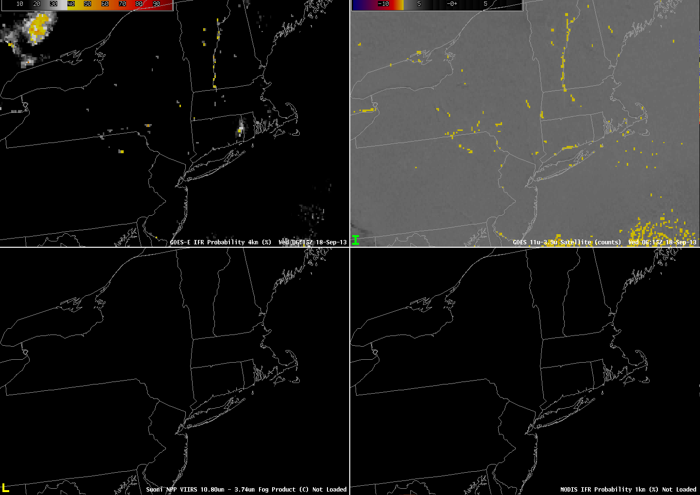
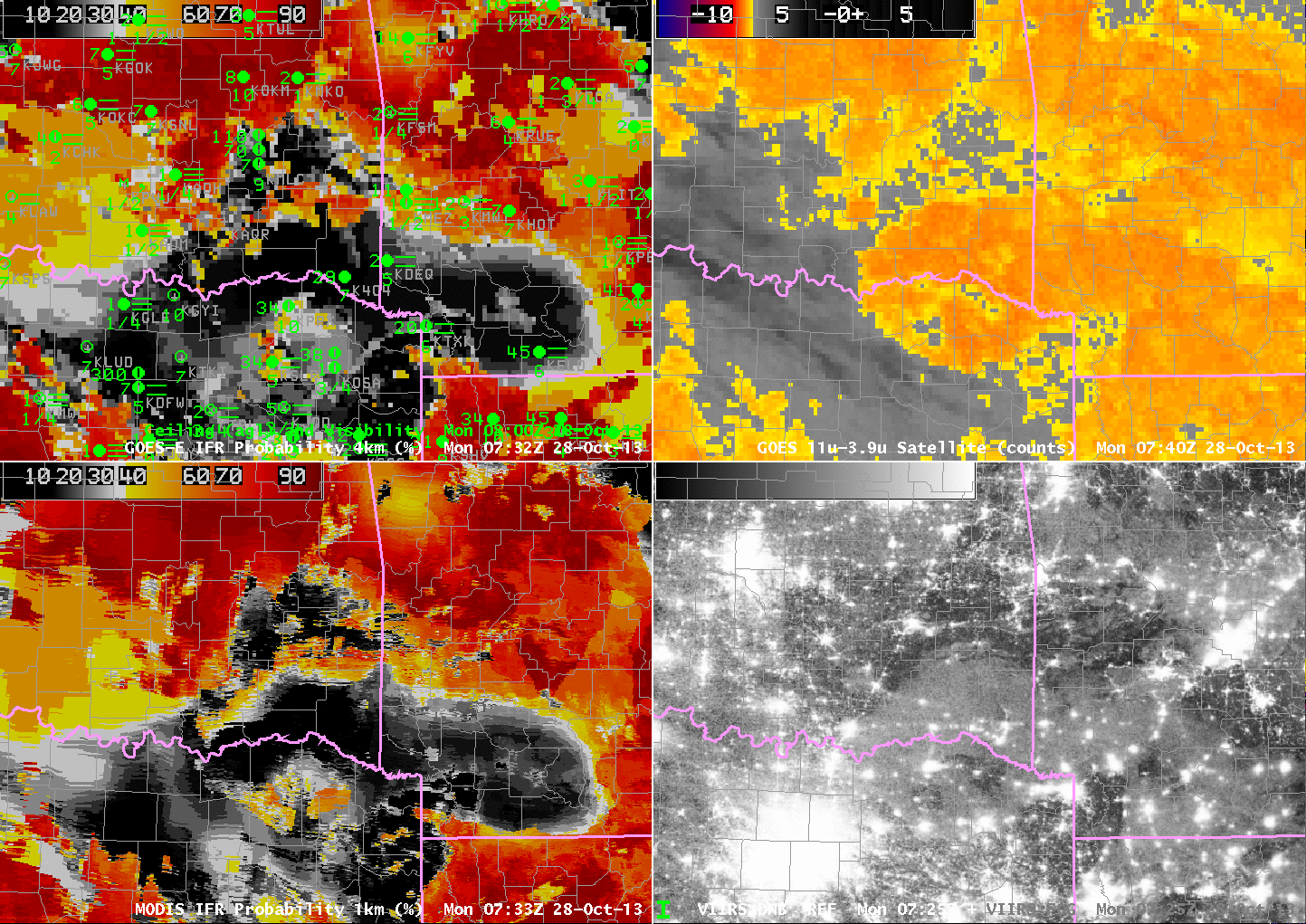
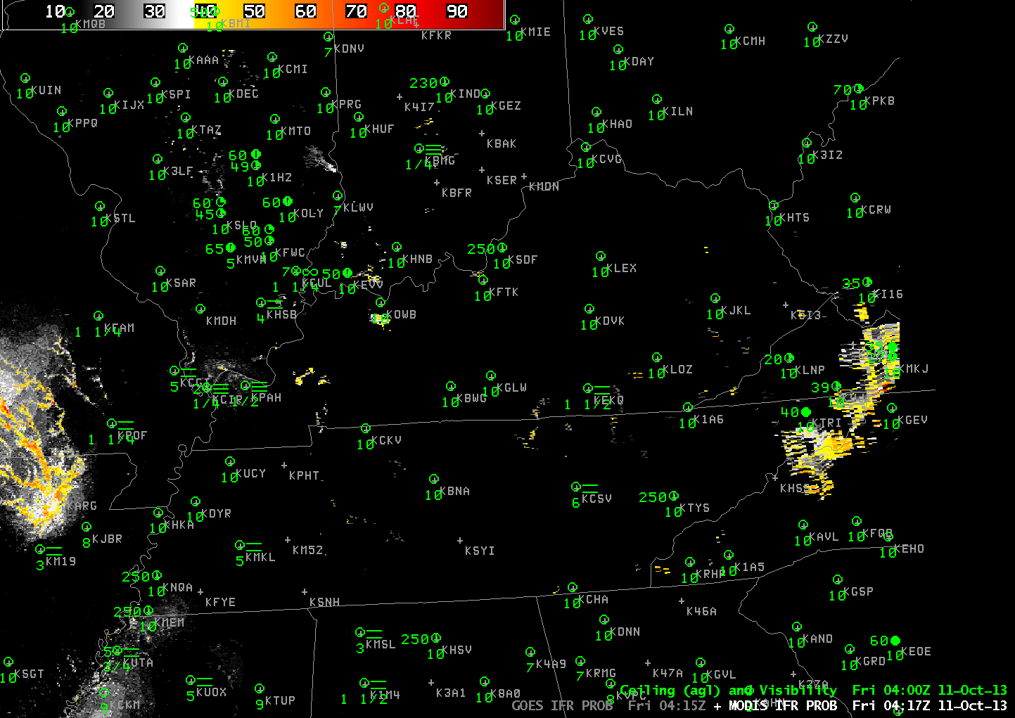
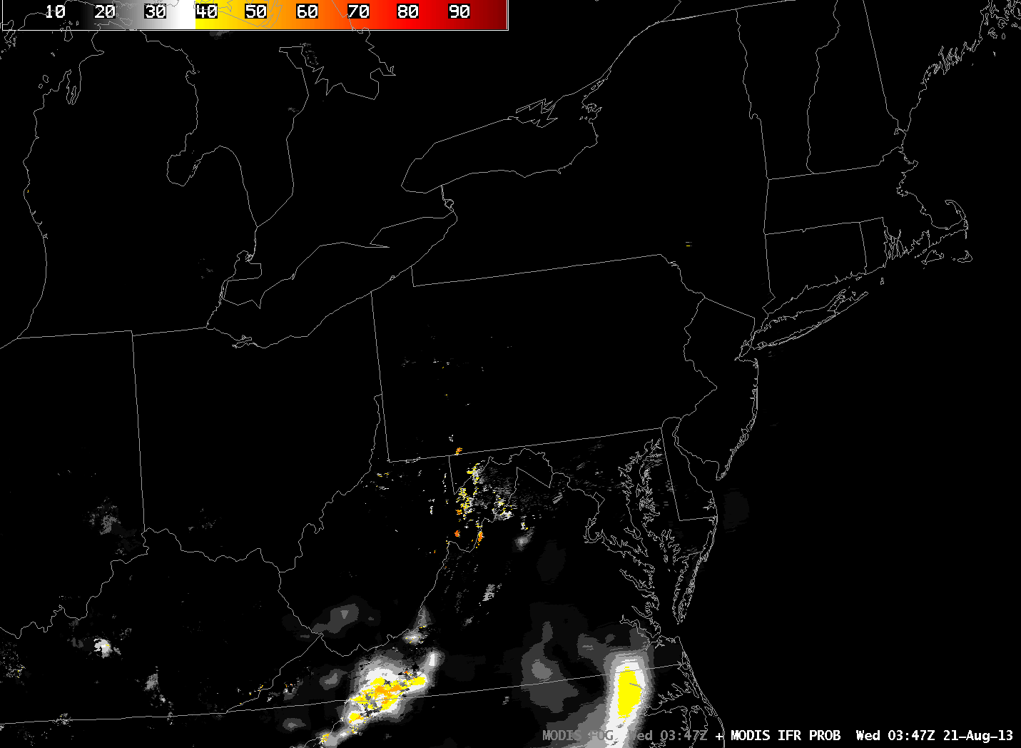
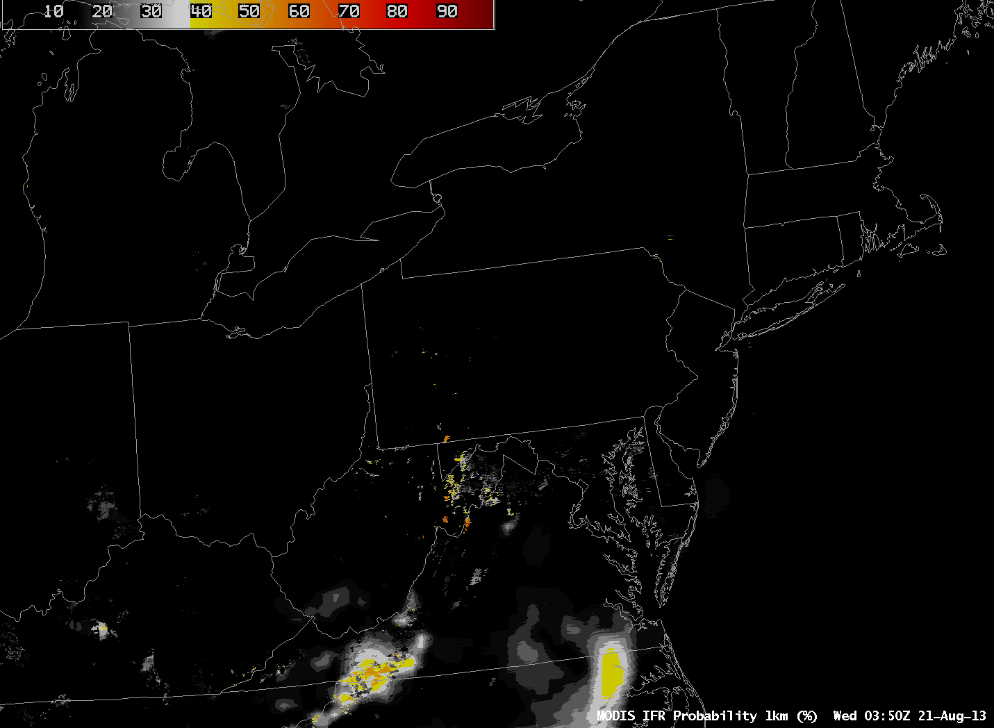
GOES-R IFR Probability (Upper Left), GOES-East Brightness Temperature Difference (Upper Right), Suomi/NPP Brightness Temperature Difference (Lower Left), MODIS-based IFR Probability (Lower Right), all imagery at 0615 UTC on 18 September 2013 (click image to enlarge)

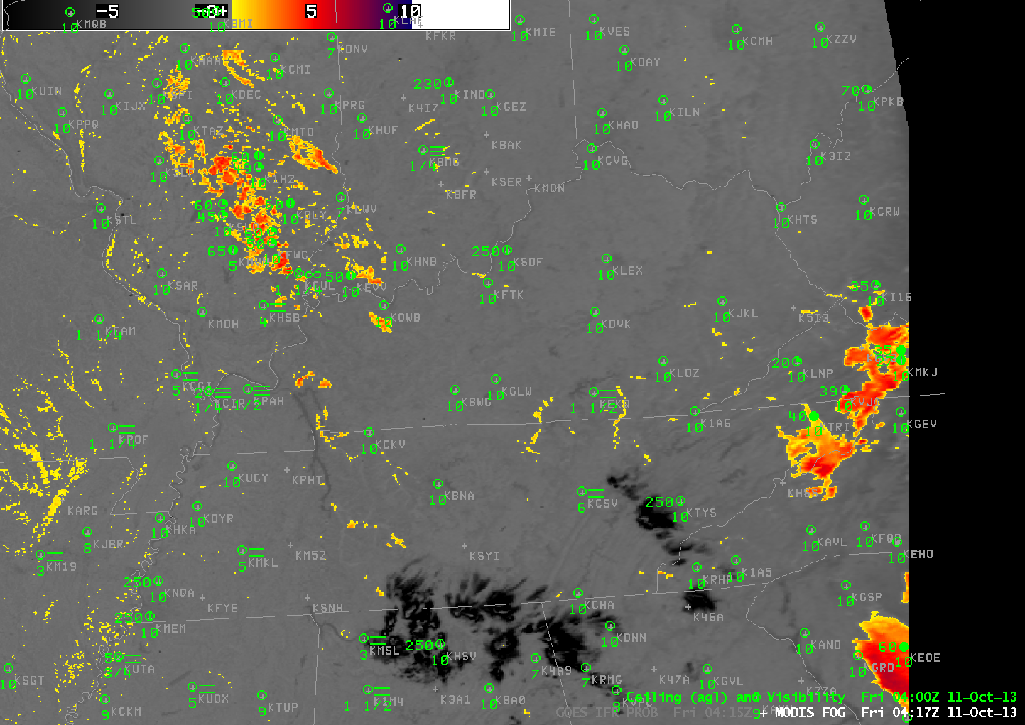
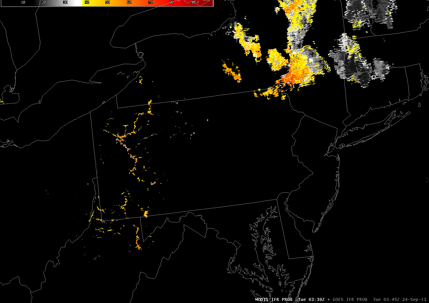
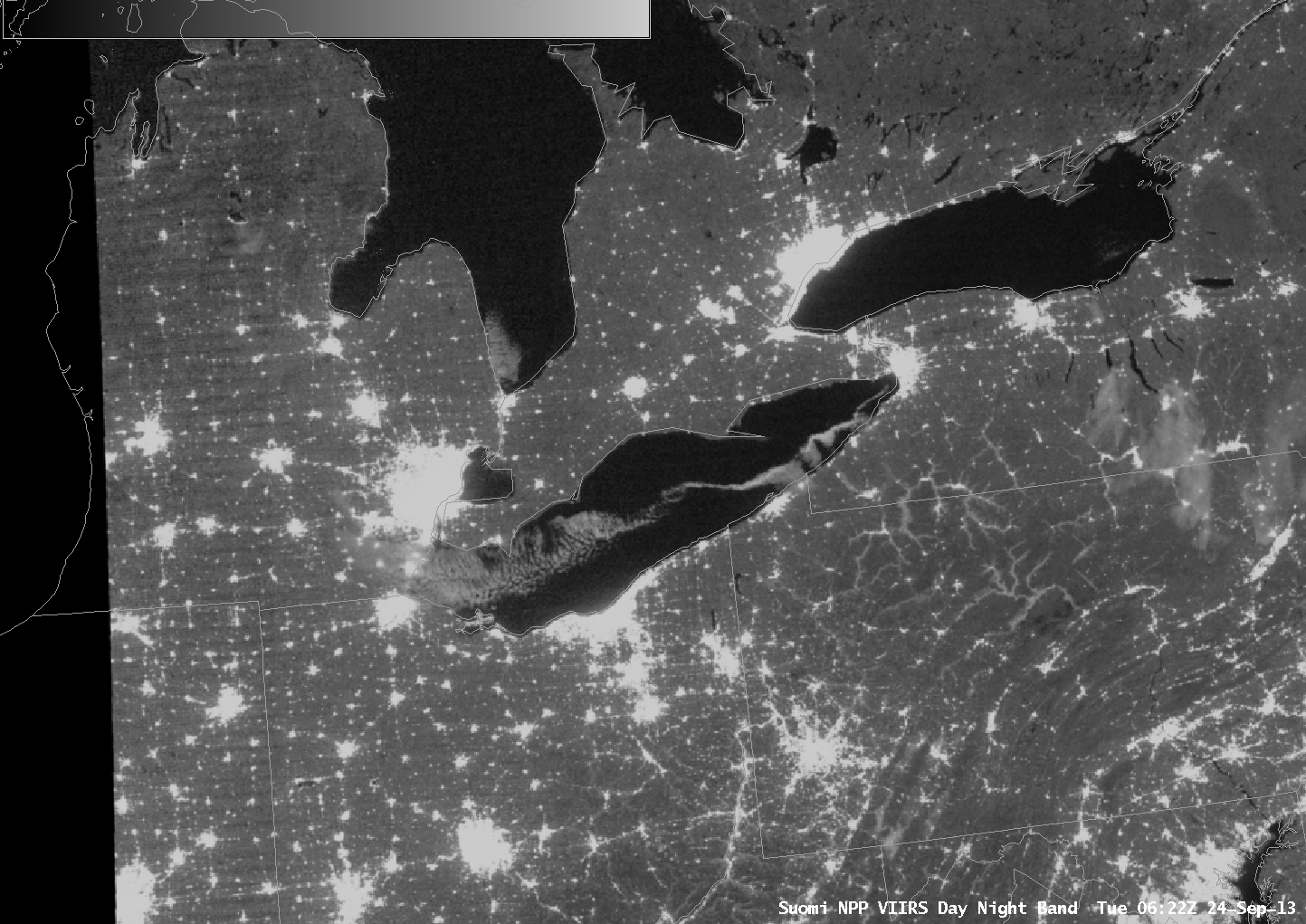
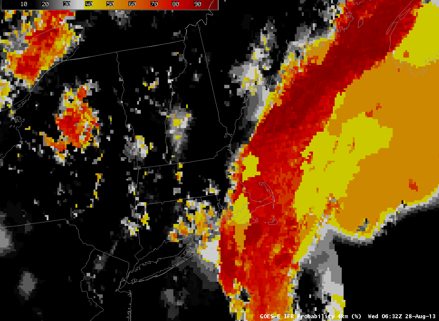
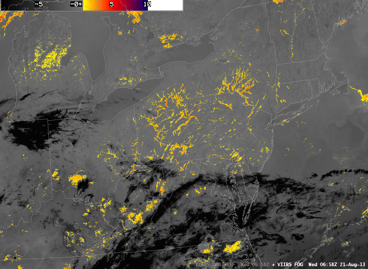
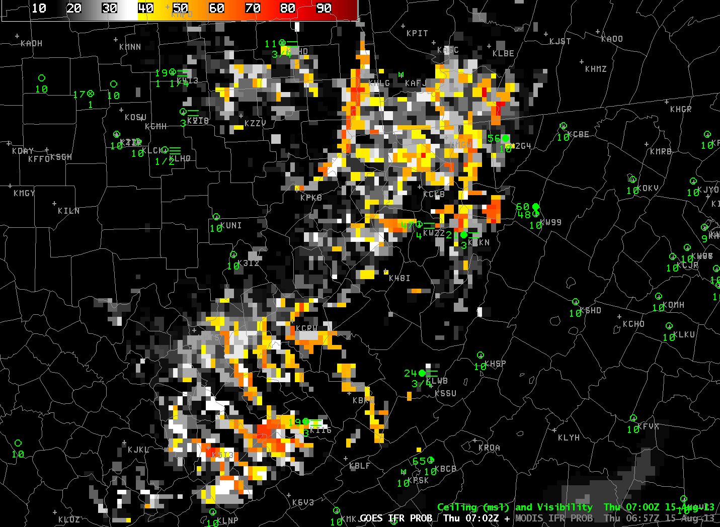
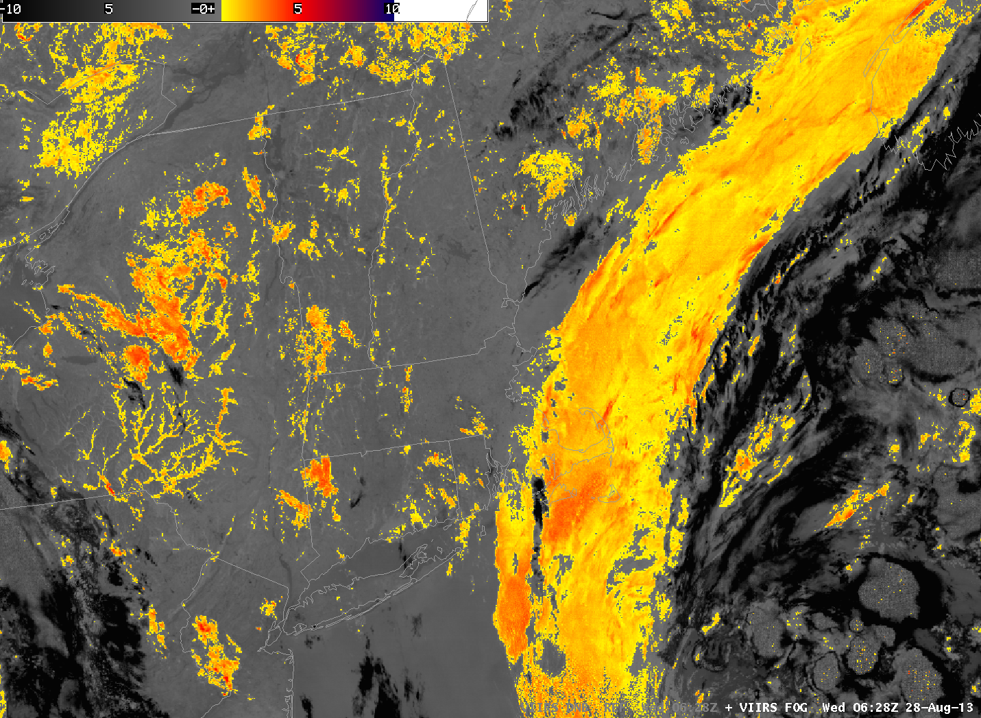
Nominal GOES resolution for the Brightness Temperature Difference product that is used in the GOES-R IFR Probability is 4 km at the sub-satellite point, and it worsens as you move into mid-latitudes. Rapid Refresh Model resolution is even coarser than the satellite. When fog is forming in narrow valleys, then, there can be a significant lag in the time from when it starts to form to when the satellite data, and the satellite/model fused product, detects it. In the 0615 UTC image above, for example, only a few pixels of strong GOES-detected Brightness Temperature Difference, and enhanced IFR Probabilities, exist. In the 0630 UTC image, below, there has been little change in the GOES-based imagery. However, the Suomi/NPP data at the time, at 1-km resolution, suggests fog is forming in many of the river valleys of Pennsylvania, but it is still sub-gridscale as far as GOES can detect.

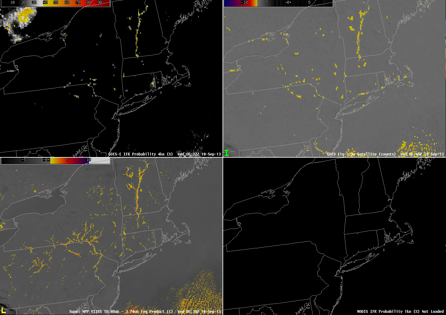
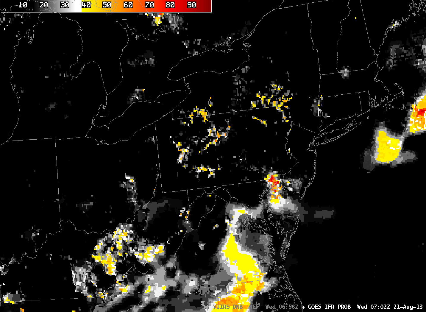
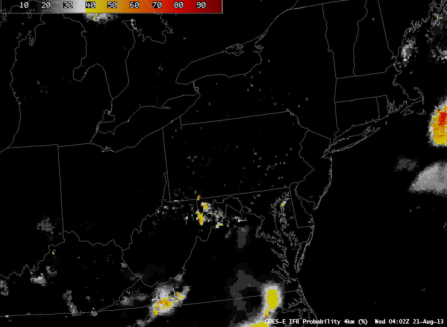
GOES-R IFR Probability (Upper Left), GOES-East Brightness Temperature Difference (Upper Right), Toggle between Suomi/NPP Day/Night band imagery and Suomi/NPP Brightness Temperature Difference (Lower Left), MODIS-based IFR Probability (Lower Right), all imagery at ~0630 UTC on 18 September 2013 (click image to enlarge)

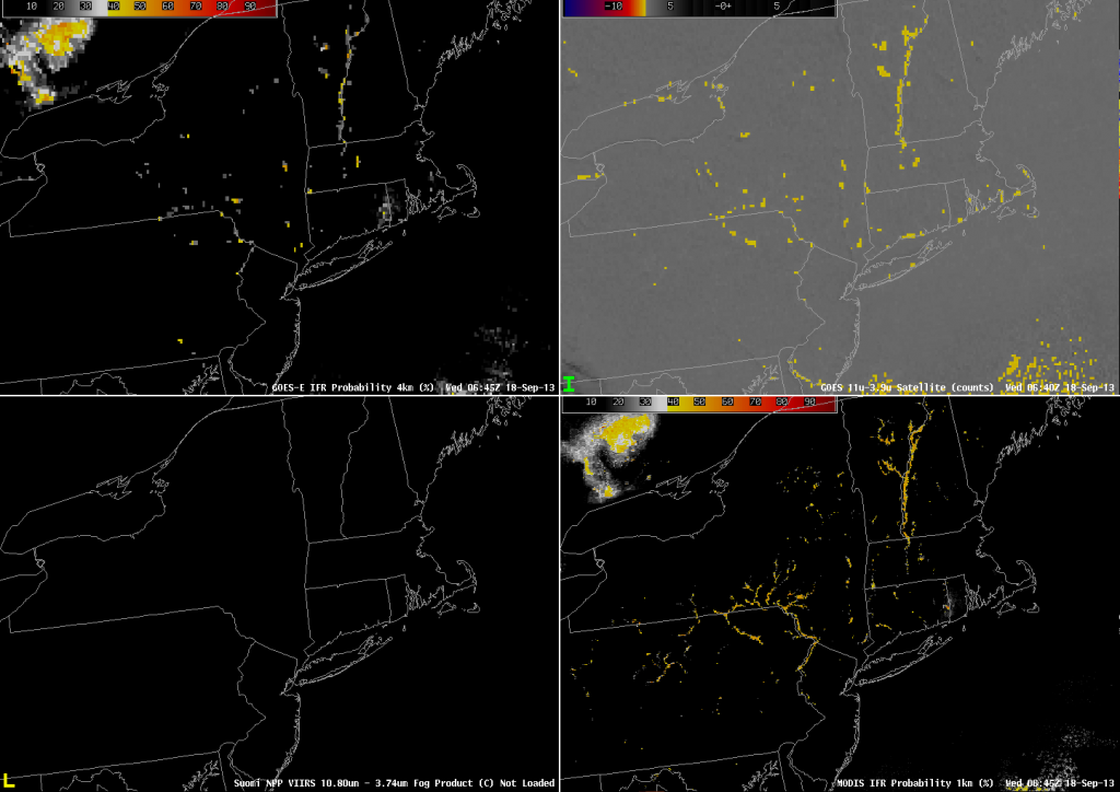
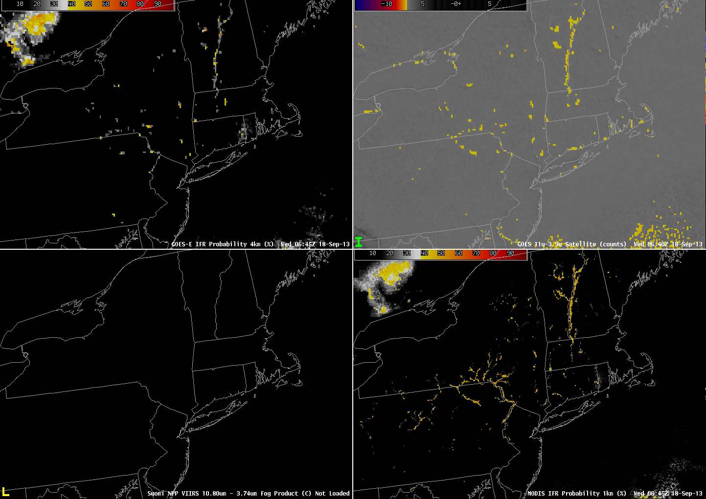
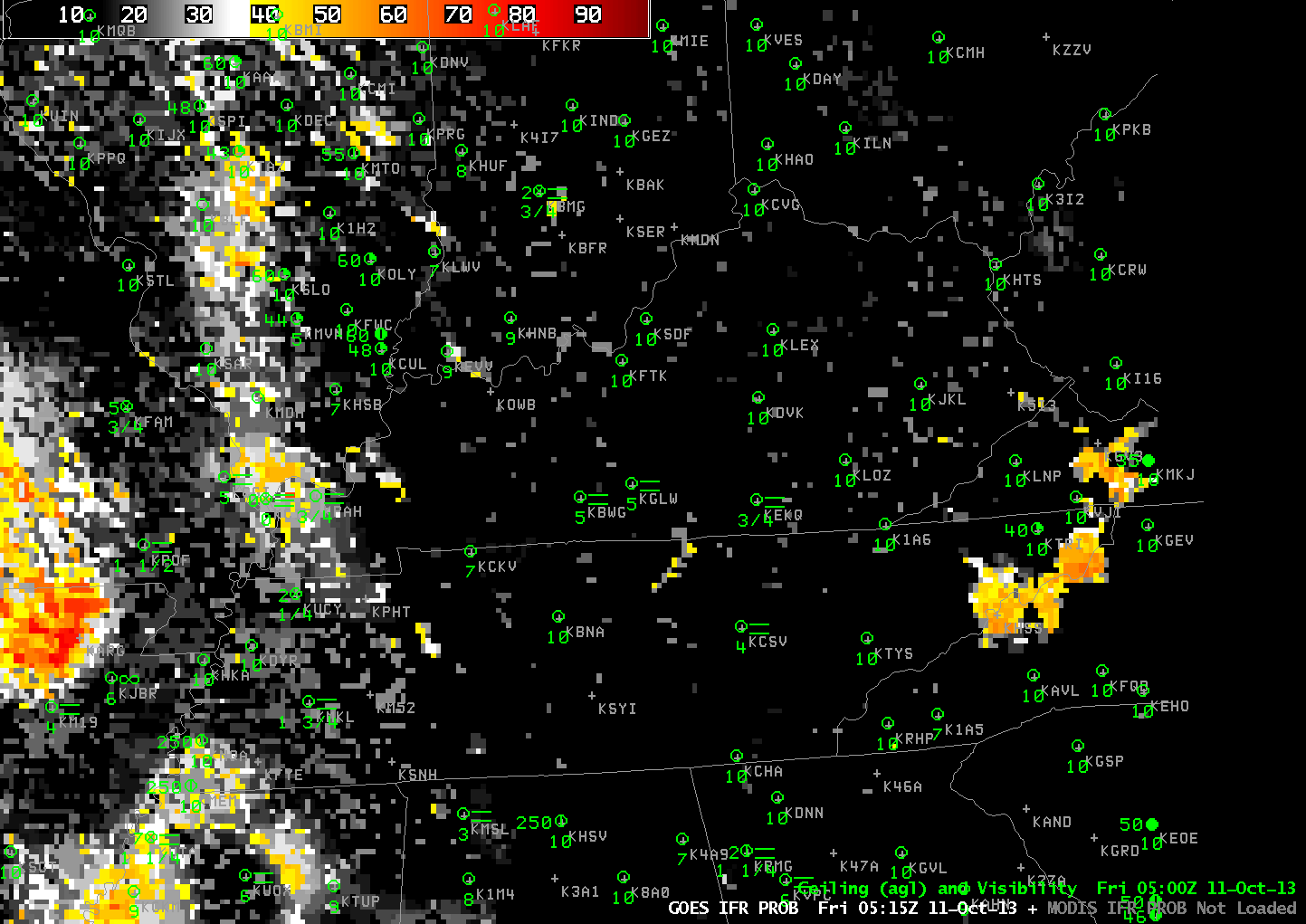
GOES-R IFR Probability (Upper Left), GOES-East Brightness Temperature Difference (Upper Right), Suomi/NPP Brightness Temperature Difference (Lower Left), MODIS-based IFR Probability (Lower Right), all imagery at 0645 UTC on 18 September 2013 (click image to enlarge)

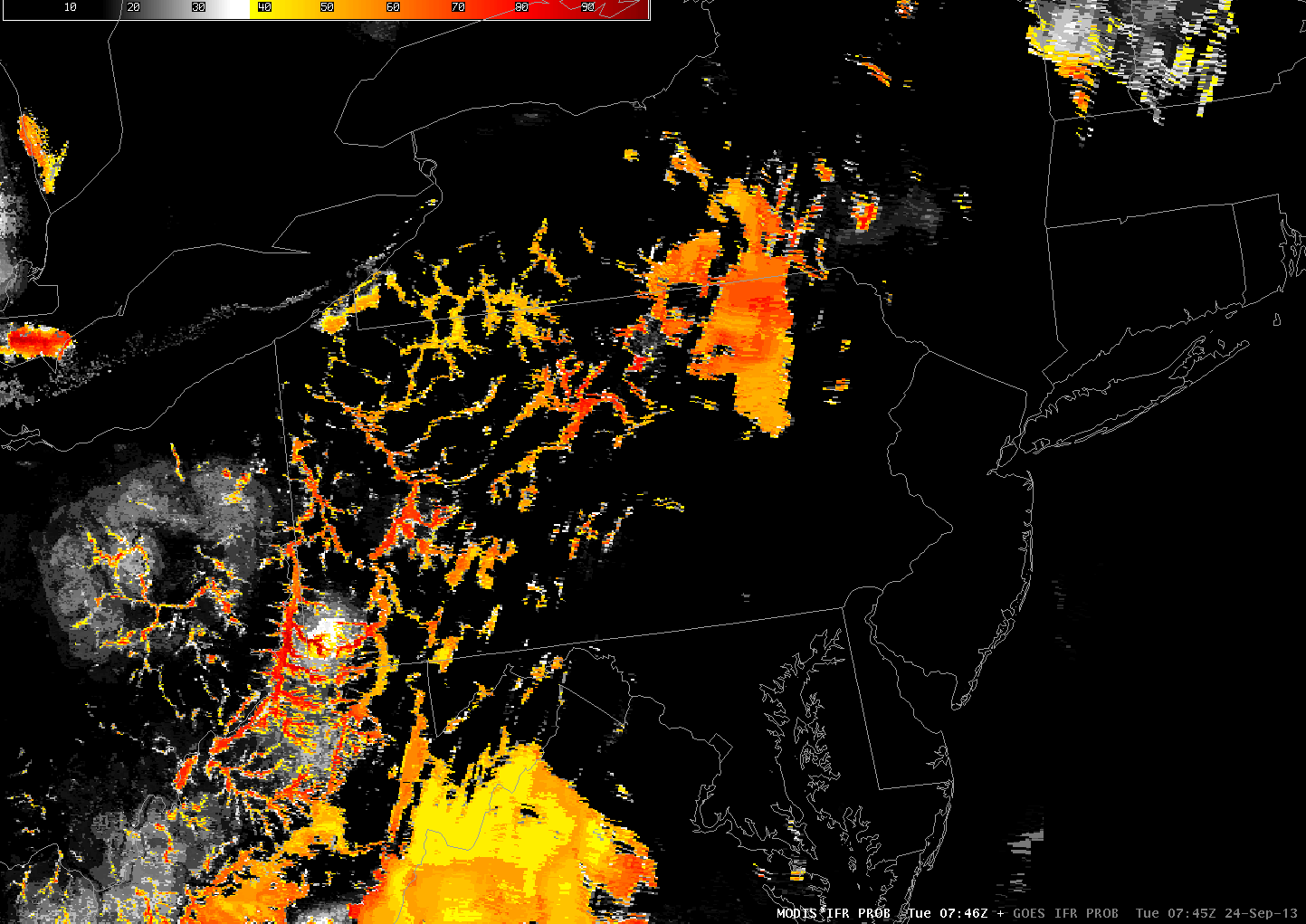
Fifteen minutes later, the MODIS-based IFR probabilities (above) suggest a strong possibility of IFR conditions in many of the river valleys of Pennsylvania. However, Suomi/NPP and MODIS data come from polar orbiters so that high resolution information is infrequent. When GOES-R is launched, ABI will have nominal 2-km resolution in the infrared, which resolution is intermediate between GOES and MODIS.

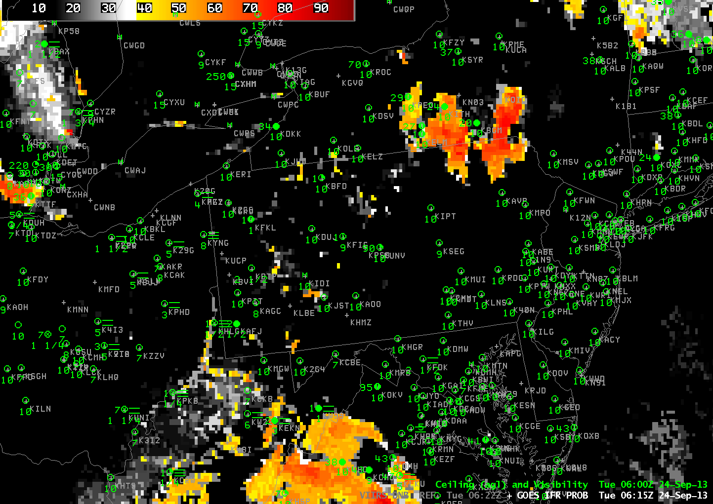
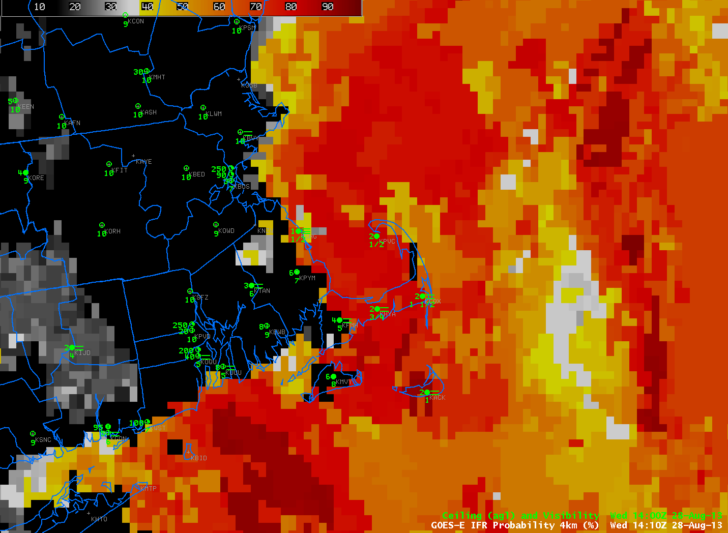
The higher-resolution polar orbiters’ occasional views can give a forecaster an important heads’ up for fog formation. By 0815 UTC the GOES-based information is showing higher IFR probabilities in the river valleys of Pennsylvania, but a Suomi/NPP overpass shows that it is still underestimating the areal extent of the fog.

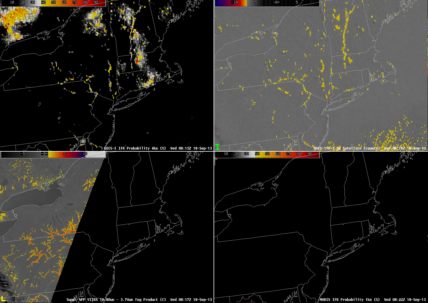
GOES-R IFR Probability (Upper Left), GOES-East Brightness Temperature Difference (Upper Right), Toggle between Suomi/NPP Day/Night band imagery and Suomi/NPP Brightness Temperature Difference (Lower Left), MODIS-based IFR Probability (Lower Right), all imagery at ~0815 UTC on 18 September 2013 (click image to enlarge)

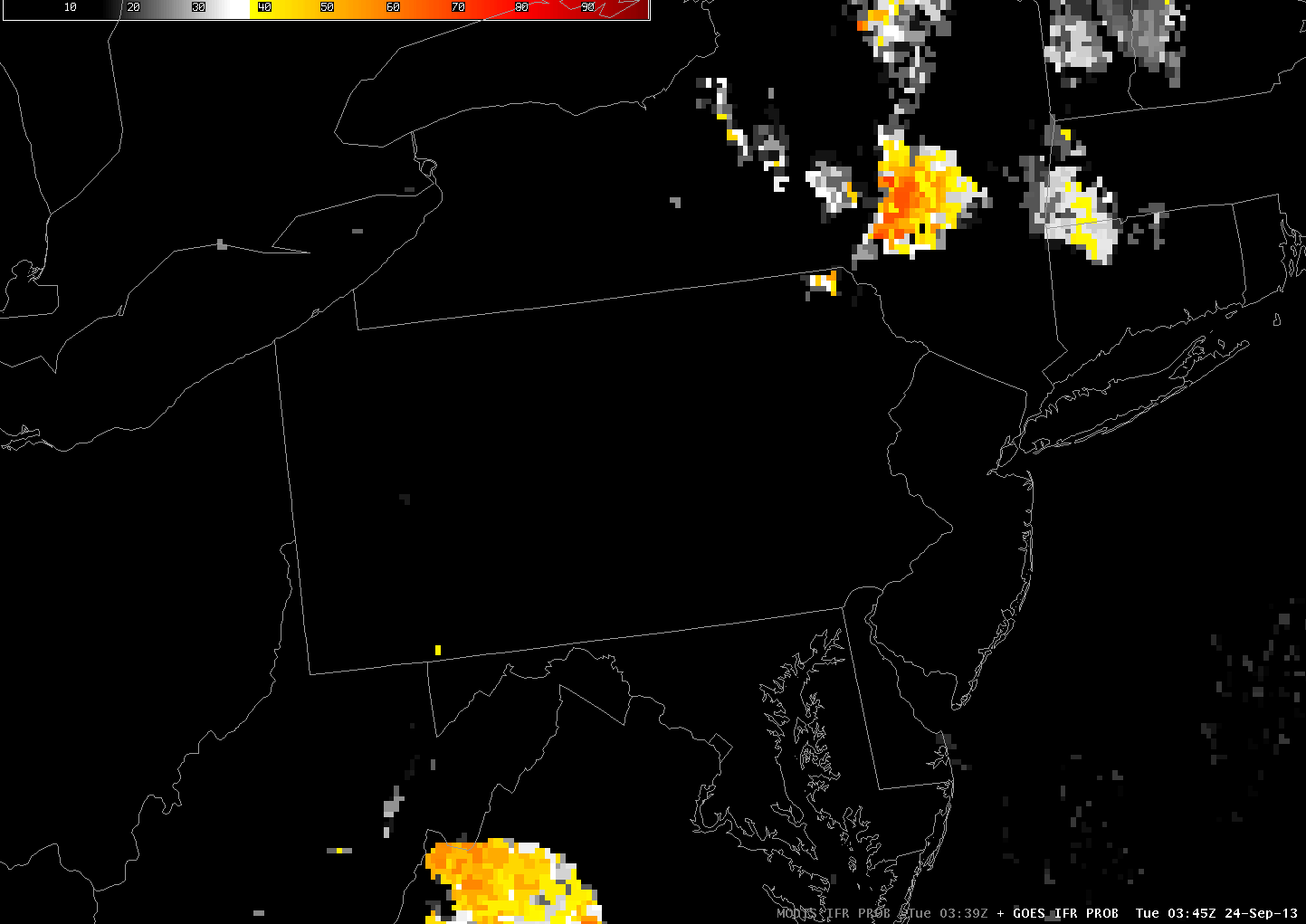
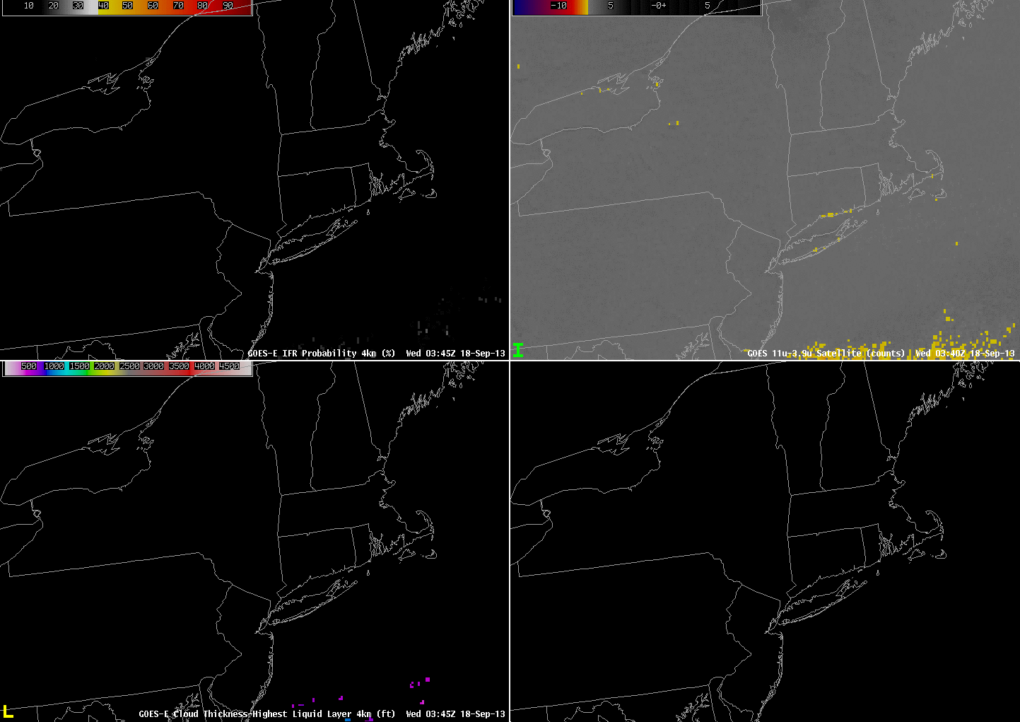
Note that this is a time of year when stray light does occasionally enter the GOES signal, causing contamination. This occurred — and was very obvious — around 0400 UTC on 18 September. As is typical, it was present for only one scan. See below.

GOES-R IFR Probability (Upper Left), GOES-East Brightness Temperature Difference (Upper Right), GOES-R Cloud Thickness (Lower Left), MODIS-based IFR Probability (Lower Right), all imagery at ~0815 UTC on 18 September 2013 (click image to enlarge)

Fog on Cape Cod

Fog developed over Cape Cod and the Islands overnight into the early morning on August 28th. The animation above (click image to animate) shows high IFR probabilities over land adjacent to the ocean. Observations show IFR or near-IFR conditions in these regions. IFR conditions decreased after sunrise. By 1410 UTC, the final image in the loop, IFR conditions persisted mostly only over Nantucket and Cape Cod east of Falmouth. This is where highest IFR probabilities persisted. The GOES-based IFR Probabilities suggest a sharp edge to the lowest visibilities over far eastern Massachusetts, which edge was just east of a Newport (RI) to Taunton (MA) line. MODIS-based IFR probabilities at 0218 UTC, below, also suggest a sharp western edge to the IFR conditions.

VIIRS data from Suomi/NPP includes both the Day/Night Band and a Brightness Temperature Difference. These data are toggled with the GOES-based IFR Probabilities below. Resolution limitations inherent with GOES data preclude the accurate detection of fog in small river valleys.

Valley Fog in Pennsylvania

The above animation bewteen the Suomi/NPP VIIRS Day/Night Band and the brightness temperature difference between the longwave infrared image and the shortwave infrared image (that highlights water-based clouds because of emissivity differences at the two wavelengths) shows fog/low stratus in the river valleys of Pennsylvania. The high spatial resolution of Suomi/NPP allows remarkable detail, and the near-Full Moon provides ample illumination. How well did more conventional satellite imagery depict the developing fog? The GOES-13-based IFR Probability Field, below, shows relatively high values in regions over Pennsylvania that are near the river valleys, but GOES lacks the spatial resolution to portray adequately the horizontally confined river valley fog — although someone with knowledge of Pennsylvania Geography can infer a lot.

The strength of GOES imagery is temporal consistency and 15-minute timesteps. Polar orbiter data can only give occasional looks. For example, MODIS Imagery can be used to generate brightness temperature differences and IFR Probabilities, below, but they are produced only every 90 minutes at most (although they will still give useful information, even at the edges of the MODIS swath where resolution is degraded).

The animation of IFR Probabilities from GOES-East, below, nicely depicts the slow increase in Valley Fog. This animation in concert with knowledge of the geography, augmented with the occasional high-resolution imagery from polar orbiters, as above, should allow a forecaster to describe the location of fog development overnight.

Visible imagery, below, shows the dissipation of the fog during the morning of August 21st.

Fog was also abundant over Pennsylvania the morning of 20 August. GOES-14, in SRSO-R mode, captured the dissipation. Link. (Courtesy Dan Lindsey, NOAA).

What does MODIS-type Resolution get you?

MODIS-based IFR Probabilities and Cloud Thickness, 0657 UTC on 15 August 2013

The 1-km data available from the MODIS (above) that is on the Terra and Aqua satellites allows much better resolution than the nominal 4-km resolution from GOES-East and GOES-West (below). The higher resolution on MODIS yields better depiction of dendritic valley fog patterns in mountainous regions. Extremes in cloud thickness will be deeper with MODIS data as well. (In this example, MODIS-based cloud depths reach 1300 feet, vs. 900 feet in GOES) In addition, because fog/low stratus generally starts at small scales and grows in size, MODIS is more likely to detect the early stages of fog (if a serendipitous overpass occurs). Thus, a forecaster can be alert to subsequent development in the GOES data with its better temporal resolution.

GOES-based IFR Probabilities and Cloud Thickness, 0657 UTC on 15 August 2013

GOES-based IFR Probabilities and Cloud Thickness, 0702 UTC on 15 August 2013

GOES-R Fog Product Examples

Fog detection fusing GOES, Terra/Aqua or Suomi/NPP Satellite data with Model output