Category Archives: MODIS

IFR Conditions over the southern Plains

GOES-R IFR Probabilities from 0100 through 1500 UTC on 10 February 2014 (click image to enlarge)

Cold air dropping southward through the southern Plains is sometimes shunted westward towards higher elevation on the Equatorward side of the Polar High that anchors the cold air. That upslope flow facilitates the development of fog and low stratus. That was the case today, and the southward and westward movement of low clouds/fog is obvious in the IFR Probability field animation shown above. Much of the High Plains south of Kansas had reduced visibility and lowered ceilings, and IFR Probabilities were high.

The IFR Probability field does a better job of outlining where the low clouds associated with IFR Conditions are present. Compare the half-hourly loop above to the hourly loop of the Brightness Temperature Difference (10.7 µm – 3.9 µm), below. Regions with multiple cloud layers show little signal in the brightness temperature field, and the flip in signal at sunrise — as 3.9 µm radiation from the Sun is reflected off the clouds, overwhelming the emitted signal — is obvious.

GOES-East Brightness Temperature Difference (10.7 µm – 3.9 µm) 0300 through 1500 UTC on 10 February 2014 (click image to enlarge)

Polar-orbiting satellites can give high-resolution views of scenes. Suomi/NPP carries the VIIRS instrument, which has a Day/Night band and 11.35 and 3.74 µm channels, shown below in a toggle. Of course, these views are telling you something about the top of the clouds only. Whether of not visibility/ceiling restrictions are happening is unknown. GOES-R IFR Probability algorithms have not yet been configured for Suomi/NPP data (such a configuration is complicated by the lack of a water vapor channel on VIIRS). The characteristic signal of high clouds — dark features in the enhancement used — shows up in the VIIRS Brightness Temperature Difference field.

Suomi/NPP VIIRS Day/Night band and Brightness Temperature Difference (11.35 µm – 3.74 µm) at 0756 UTC on 10 February 2014 (click image to enlarge)

MODIS data includes water vapor imagery, and thus GOES-R IFR Probability fields can be computed using MODIS data, as shown below from 0907 UTC. This toggle includes MODIS-based Brightness Temperature Differences, MODIS-based GOES-R IFR Probabilities, GOES-based GOES-R IFR Probabilities and GOES Brightness Temperature Differences. The shortcoming of the MODIS-based data is obvious (it doesn’t view the entire scene), but its strength (excellent spatial resolution) is also apparent.

MODIS Brightness Temperature Difference (11 µm – 3.9 µm), MODIS-based GOES-R IFR Probabilities, GOES-based GOES-R IFR Probabilities and GOES-East Brightness Temperature Differences (10.7 µm – 3.9 µm) at ~0910 UTC on 10 February 2014 (click image to enlarge)

GOES-R IFR Probability signal because of co-registration errors

GOES-R IFR Probabilities at 0802 UTC, 30 January 2014 (click image to enlarge)

Special Update, 17 November 2014.

GOES-R IFR Probabilities on the morning of 30 January suggested the likelihood of fog along some of the Finger Lakes of upstate New York. These high probabilities arise because the Brightness Temperature Difference (10.7 µm – 3.9 µm) Product, below, shows a signal there. Note, however, that the Brightness Temperature Difference has a shadow; this is the sign that the co-registration error that is present between the 10.7 µm and 3.9 µm channels is producing a fictitious signal of fog over the lake. Such errors have been discussed here and elsewhere in the past.

GOES-East Brightness Temperature Difference (10.7 µm – 3.9 µm) at 0801 UTC, 30 January 2014 (click image to enlarge)

Evidence that fog is not present is available in Suomi/NPP data taken at the same time as the GOES data, above. The toggle, below, of Day/Night Band imagery and of the brightness temperature difference (11.35 µm – 3.74 µm) from VIIRS shows scant evidence of fog/low stratus near the Finger Lakes. Because the moon is new, lunar illumination is at a minimum and surface features in the Day/Night band are not distinct, but the dark waters of the lakes are apparent.

Suomi/NPP VIIRS Day/Night band and Brightness Temperature Difference (11.35 µm – 3.74 µm) at 0802 UTC, 30 January 2014 (click image to enlarge)

MODIS data also suggests no fog/low stratus in the region. Both the brightness temperature difference field and the MODIS-based IFR Probabilities, below, support a forecast that does not mention fog around the Finger Lakes.

MODIS Brightness Temperature Difference (11 µm – 3.74 µm) and MODIS-based GOES-R IFR Probabilities at 0746 UTC, 30 January 2014 (click image to enlarge)

=====================================================================

Update, 17 November 2014

NOAA/NESDIS has tested a software fix to align better the longwave infrared (10.7 µm) and shortwave infrared (3.9 µm) channels. The toggle below is of the Brightness Temperature Difference Field with (After co-registration correction) and without (Prior to co-registration correction) the realignment.

GOES-13 Brightness Temperature Difference Fields at 0802 UTC, 30 January 2014, with and without the co-registration correction as indicated (Photo Credit: UW-Madison CIMSS; Click to enlarge)

The correction of the co-registration error translates into more realistic IFR Probabilities in/around the Finger Lakes. In this case, IFR Probabilities are reduced because the false strong signal from the satellite is not present because of more accurate co-registration.

GOES-R IFR Probability fields computed Prior to and After co-registration correction, data from 0802 UTC 30 January 2014. IFR Probability fields with the corrected co-registration data are more accurate. (Photo Credit: UW-Madison CIMSS; Click to enlarge)

Fog in Idaho, Oregon and Washington over three days

Suomi/NPP Day/Night band imagery over the Pacific Northwest, 0912 and 1053 UTC on 21 January 2014(click image to enlarge)

Suomi/NPP viewed eastern Oregon/Washington and western Idaho on two successive scans overnight. The 3/4 full moon provides ample illumination, and fog/low stratus is apparent in the imagery above. A view of the top of the clouds, however, gives little information about the cloud base, that is, whether or not important restrictions in visibility are occurring. For something like that, it is helpful to include surface-based data. Rapid Refresh data are fused with the model data to highlight regions where IFR conditions are most likely. The image below is a toggle of the 1053 UTC Day/Night band image and the 1100 UTC GOES-R IFR Probabilities (computed using GOES-West data). GOES-R IFR Probabilities are correctly highlighting regions where ceilings and visibilities are consistent with IFR conditions. Where the Day/Night band is possibly seeing elevated stratus (between The Dalles (KDLS) and Yakima (KYKM), for example), IFR Probabilities are lower.

GOES-based data cannot resolve very small-scale fog events in river valleys (over northeastern Washington State, for example). The superior spatial resolution of a polar-orbiting satellite like Suomi/NPP (or Terra/Aqua) can really help fine-tune understanding of the horizontal distribution of low clouds.

Suomi/NPP Day/Night band imagery and GOES-R IFR Probabilities, ~1100 UTC on 21 January 2014(click image to enlarge)

Added: 22 January 2014

Suomi/NPP Day/Night band imagery over the Pacific Northwest, 0854 and 1034 UTC on 22 January 2014(click image to enlarge)

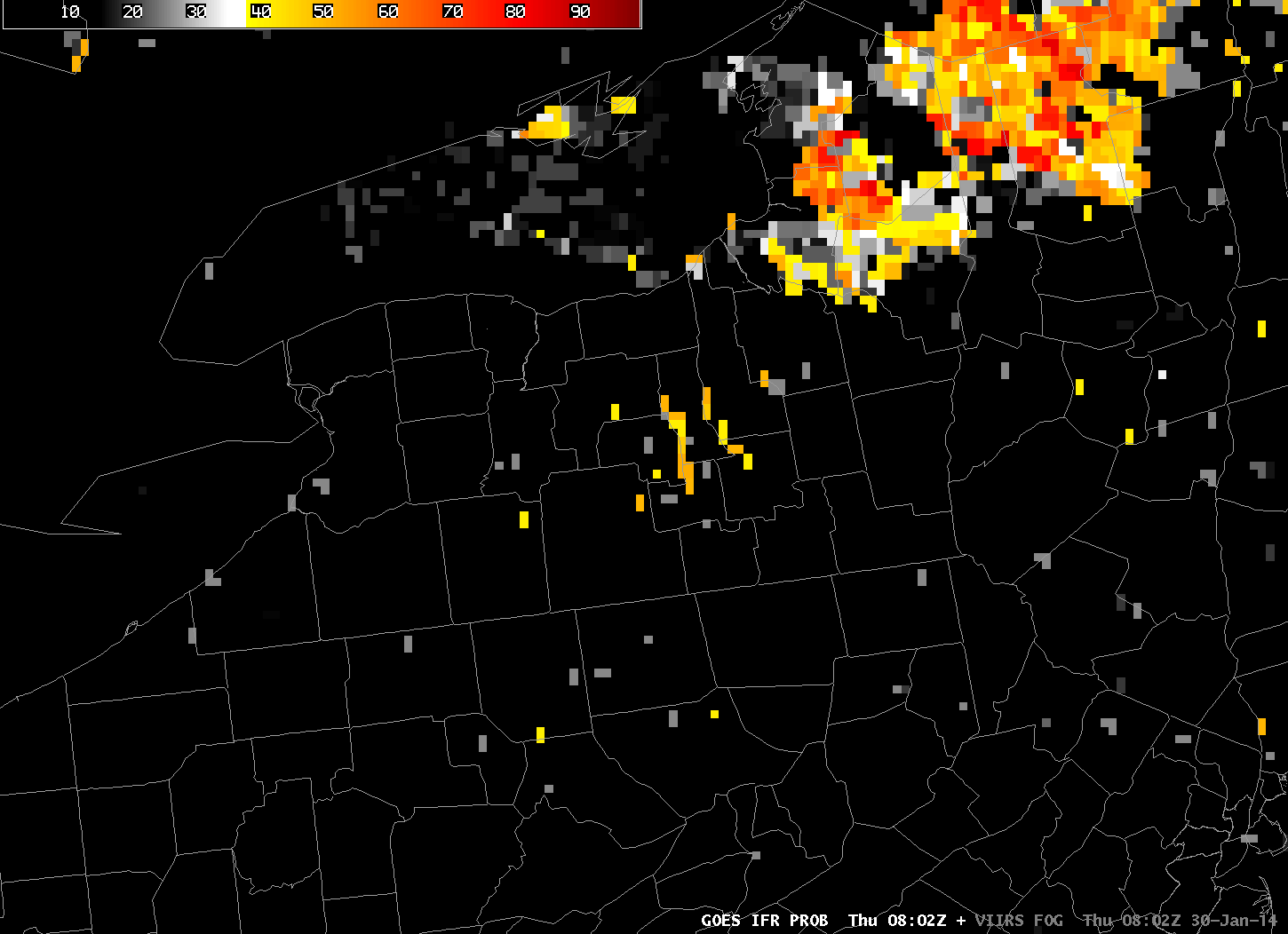
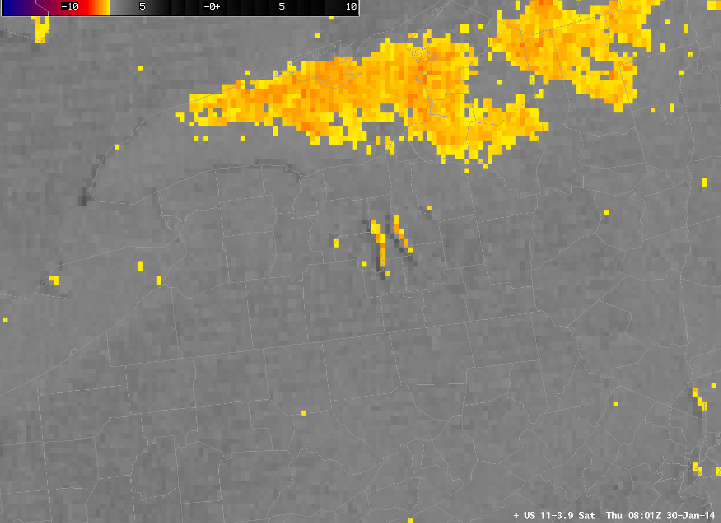
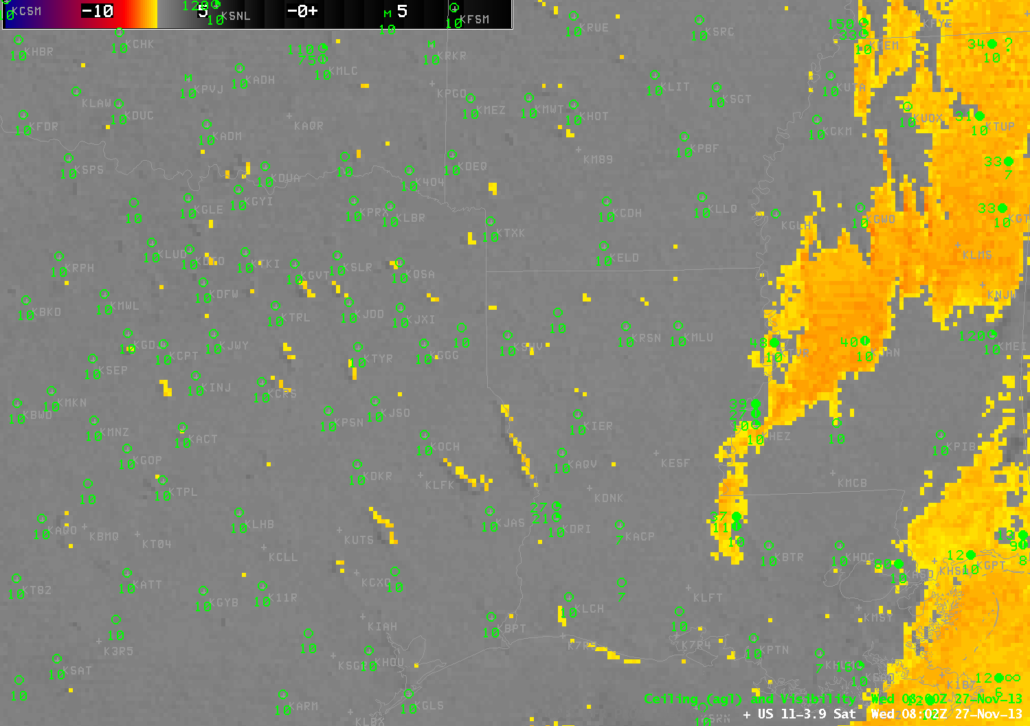
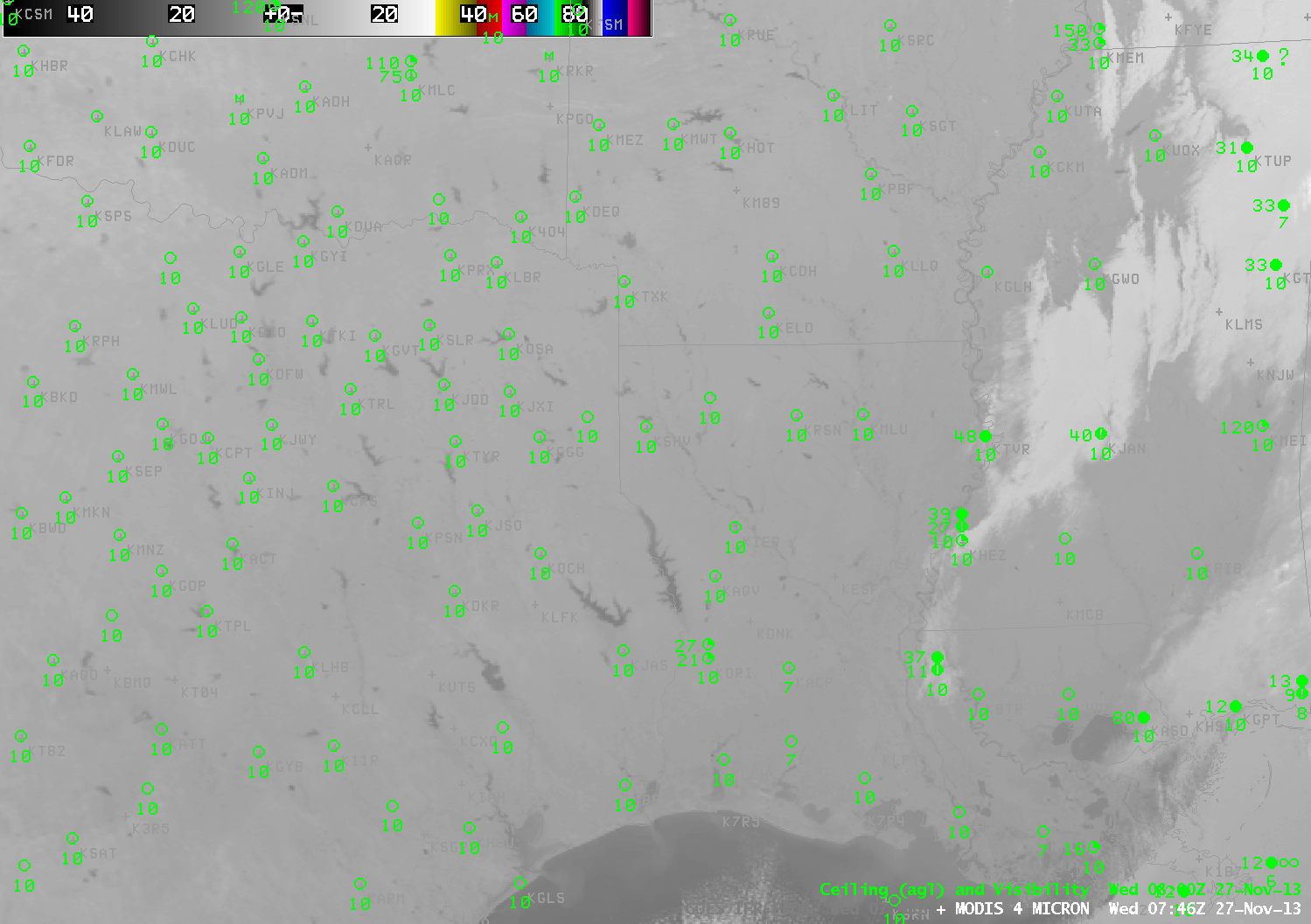
Suomi/NPP Brightness Temperature Difference from VIIRS, 11 µm – 3.74 µm imagery over the Pacific Northwest, 0854 and 1034 UTC on 22 January 2014(click image to enlarge)

The stagnant weather pattern under the west coast ridge allowed fog to persist overnight on January 22nd, and once again, the Day/Night band observed the fog-filled Snake River Valley of southern Idaho. The newly-rising moon at 0854 UTC provided less illumination than the higher moon at 1034 UTC, but both show fog/low stratus over the Snake River Valley of Idaho, and over parts of northern Oregon and central Washington. It is difficult to tell where the stratus is close enough to the ground to produce IFR conditions, however. The brightness temperature difference product from VIIRS, above, can distinguish between low clouds (orange enhancement) and higher clouds (dark grey) because of the different emissivity properties of water-based low clouds and ice-based higher clouds.

The toggle below shows how the higher-resolution VIIRS instrument can more accurately portray sharp edges to low clouds. Both instruments show the region of high clouds moving onshore in coastal Oregon (at the very very edge of the Suomi/NPP scan). These high clouds make satellite-detection of low clouds difficult because they mask detection of lower clouds.

Suomi/NPP Brightness Temperature Difference from VIIRS (10.35 µm – 3.74 µm) and GOES-15 Imager Brightness Temperature Difference (10.7 µm – 3.9 µm imagery over the Pacific Northwest, ~0900 UTC on 22 January 2014(click image to enlarge)

GOES IFR Probabilities at 0900 UTC and at 1030 UTC (click image to enlarge)

GOES-based IFR Probabilities show the probability of fog and low ceilings (IFR conditions) even where high clouds are present. In the toggle above, note the regions where the IFR Probability field is uniform (off the coast of Oregon, yellow, and over west-central Washington State, orange and yellow, both at 0900 UTC). These smooth fields are typical of IFR Probabilities that are determined primarily from Rapid Refresh data. Where those smooth fields exist, satellite data does not give a signal of low clouds — usually because of the presence of ice-based clouds at higher levels; therefore, model data are driving the IFR Probability signal, and model data are typically smoother than the more pixelated satellite field. There are places, however, where model data alone does not accurately portray IFR conditions (at KGPI, for example (Glacier Park), where high clouds are present).

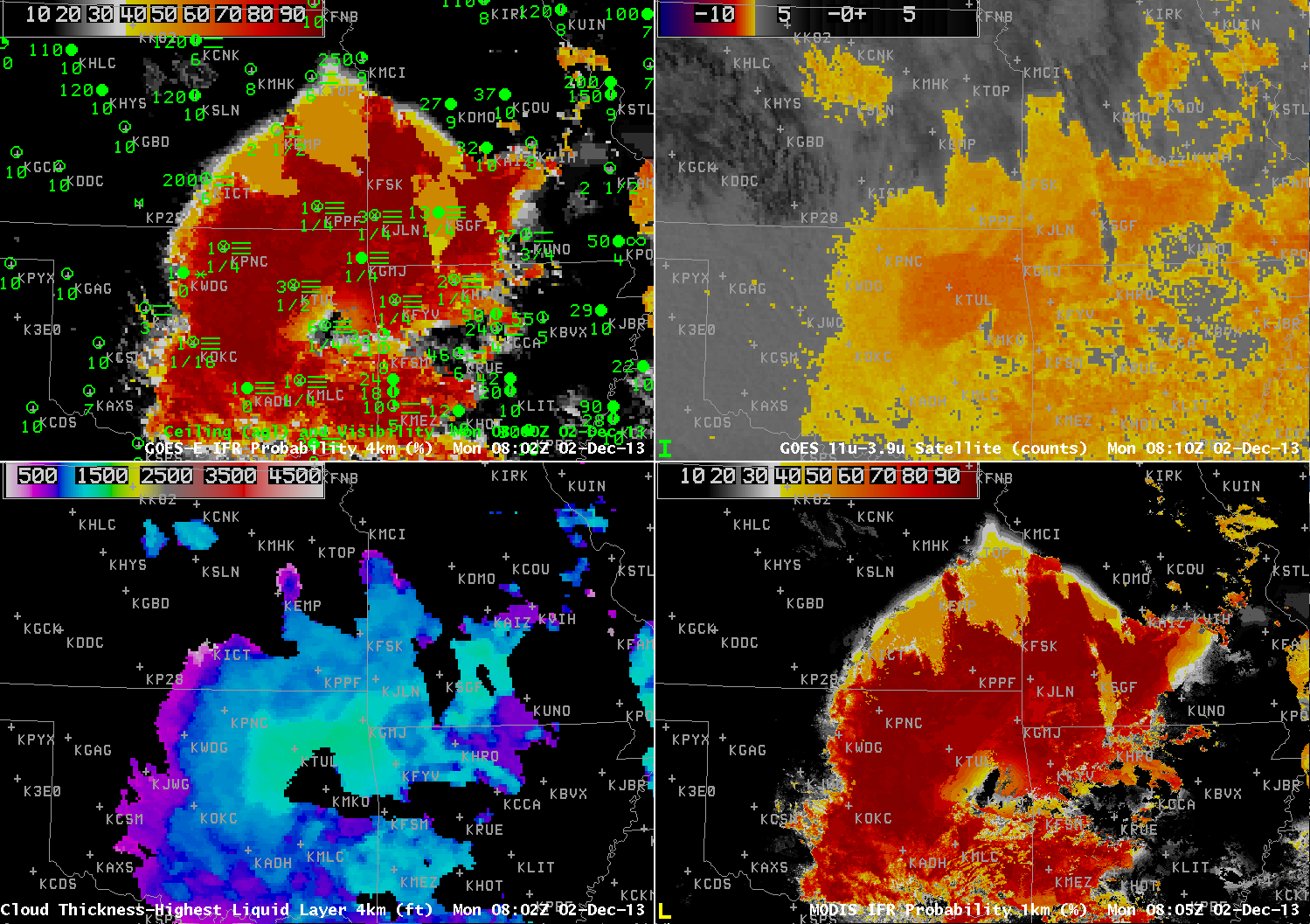
IFR Probability algorithms have not yet been extended using data from Suomi/NPP, in large part because the VIIRS instrument does not detect radiation in the so-called water-vapor channel (around 6.7 µm). The MODIS detector on board Terra and Aqua does have a water vapor channel, and IFR Probabilities are routinely produced from MODIS data, as shown below. MODIS, like VIIRS, has a 1-km pixel footprint that excels at detecting very fine small-scale features in clouds, especially small valleys, that are smeared out in the GOES imagery. The toggle below is of MODIS Brightness Temperature Difference, MODIS-based IFR Probabilities, GOES Brightness Temperature Difference, and GOES-based IFR Probabilities, all at ~1015 UTC on 22 January. Two things to note: MODIS has cleaner edges to fields, related to the high spatial resolution. The GOES-based brightness temperature difference highlights many more pixels over central Oregon where fog is not present. These positive hits bleed into the GOES-based IFR Probabilities, and they occur because of emissivity differences in very dry soils (See for example, this post). As drought conditions persist and intensify on the west coast under the longwave ridge, expect this signal to persist. The signals are not apparent in MODIS or VIIRS brightness temperature differences because of the narrower spectrum of those observations.

MODIS Brightness Temperature Difference (11 µm – 3.74 µm), MODIS-based GOES-R IFR Probabilities, GOES-15 Imager Brightness Temperature Difference (10.7 µm – 3.9 µm), GOES-based GOES-R IFR Probabilities and MODIS-based IFR Probabilities (again), all near 1015 UTC 22 January 2014(click image to enlarge)

Added, 23 January:

Fog persists in the Snake River Valley and elsewhere. It has also become more widespread over the high plains of Montana. Note the difference in the Day/Night band imagery below. At 0834 UTC, the rising quarter moon is unable to provide a lot of illumination; by 1015 UTC, however, the moon is illuminating the large areas of fog. Because the moon is waning, however, Day/Night band imagery will become less useful in the next week. A toggle between the 1015 UTC Day/Night band and the GOES-R IFR Probabilities computed using GOES-West (below the Day/Night band imagery) continues to demonstrate how well the field outlines the region of IFR conditions.

Suomi/NPP Day/Night band imagery over the Pacific Northwest, 0834 and 1015 UTC on 23 January 2014(click image to enlarge)

Suomi/NPP Day/Night band imagery and GOES-R IFR Probabilities (from GOES-15 and Rapid Refresh data) over the Pacific Northwest, 1015 UTC on 23 January 2014(click image to enlarge)

Use MODIS data at High Latitudes

GOES-West IFR Probabilities, MODIS IFR Probabilities and surface topography over northern Alaska, ~2000 UTC on 14 January 2014 (click image to enlarge)

GOES pixels grow to large sizes at high latitudes, such as those found over northern Alaska. Consequently, the IFR Probabilities can give information that is difficult to interpret. Data from the polar-orbiting MODIS instrument (on board Aqua and Terra satellites), in contrast, have nominal 1-km resolutions even at high latitudes. In the toggle of imagery above, the MODIS IFR Probabilities suggests low clouds just north of the Brooks Range in northern Alaska. In contrast, the IFR Probabilities based on GOES-15 are difficult to interpret.

Consider using the MODIS-based IFR Probabilities. At very high latitudes, data from polar orbiters is more frequent than at mid-latitudes. Thus, there is a benefit from higher spatial resolution without an onerous loss of temporal resolution as happens in mid-latitudes.

Widespread Advection Fog over the Midwest

GOES-East IFR Probabilities and surface plots of visibilities/ceilings and surface analysis of dewpoint at 0202, 0402, 0615, 0802, 1002 and 1215 UTC on 10 January 2014 (click image to enlarge)

The northward movement of moist air over a snow-covered surface allowed for widespread advection fog in the midwest overnight from January 9th to 10th. The animation, above, shows GOES-R IFR Probabilities at 2-hour time steps. Included in the plots are surface observations and cloud ceilings (documenting the widespread region of IFR conditions) and the RTMA Dewpoint analysis that shows the slow northward movement of dewpoints at the surface. As this moist air moves over the cold snow-covered surface (the snow analysis from the National Operational Hydrological Remote Sensing Center is below), advection fog is a result. The GOES-R IFR Probability fields do a fine job of outlining where the IFR conditions are observed.

Analysis of snow depth from NOHRSC, 0600 UTC, 10 January 2014 (click image to enlarge)

Note in the animation above how the presence of higher clouds moving up from the southwest affects the IFR Probability fields. As high clouds overspread the advection fog, satellite data can no longer be incorporated into the GOES-R IFR probability algorithm, and IFR Probabilities drop, in this case from values near 90% to values near 55%.

Polar-orbiting data can also give information about low clouds and fog. Temporal resolution is far superior to geostationary, as shown below. In cases of small-scale fog, polar orbiter data can give important information by identifying the first region of a developing fog. In large-scale cases such as this, high-resolution data can better identify edges to the fields. The MODIS data in this case does show high probabilities over the midwest; the brightness temperature difference field shows evidence of high clouds from central Iowa southwestward. As with the GOES data, the presence of high clouds results in lower IFR Probabilities.

Toggle between MODIS-based IFR Probabilities and Brightness Temperature Difference at 0814 UTC 10 January 2014 (click image to enlarge)

Suomi/NPP data, below, from the Day/Night band shows widespread cloudiness over the midwest. The clouds are illuminated by the moon, nearly full, setting at this time in the west. Shadows are being cast by high clouds on the lower clouds over western Minnesota. The brightness temperature difference fields from Suomi/NPP are very similar to the MODIS data. In contrast to MODIS, the VIIRS instrument does not have a water vapor sensor, so the IFR Probability algorithms are not directly transferable to Suomi/NPP VIIRS data.

Toggle between Suomi/NPP Day/Night band and Brightness Temperature Difference at 0737 UTC 10 January 2014 (click image to enlarge)

Fog Detection under Cirrus

GOES-R IFR Probabilities from GOES-13 (Upper Left), GOES-13 Brightness Temperature Difference Product (10.7 µm – 3.9 µm) (Upper Right), GOES-R Cloud Thickness from GOES-13 (Lower Left), MODIS-based IFR Probabilities (Lower Right), Times as indicated (click image to enlarge)

Dense Fog developed over the southern Plains overnight, and the case demonstrates how the Fused data product is able to give a useful signal of IFR probabilities even in regions where high clouds preclude the detection of low clouds by satellite. The fog was widespread and dense enough to warrant Dense Fog Advisories from Tulsa, Norman and Topeka forecast offices. See below, for example.

000
FXUS64 KTSA 020953
AFDTSA

AREA FORECAST DISCUSSION
NATIONAL WEATHER SERVICE TULSA OK
353 AM CST MON DEC 2 2013

.DISCUSSION…
DENSE FOG CONTINUES THIS MORNING ACROSS MUCH OF THE CWA. GIVEN THE
TIME OF YEAR /LOW SUN ANGLE/ AND THE FACT THAT SOME HIGH CLOUDS ARE
STREAMING INTO THE AREA FROM THE NW /REDUCED INSOLATION AND
DELAYED MIXING/…THINK IT MAY TAKE A LITTLE LONGER THAN
PREVIOUSLY EXPECTED TO GET RID OF THE FOG. WE HAVE EXTENDED THE
DENSE FOG ADVISORY UNTIL 11 AM. ONCE THE FOG BURNS OFF…SHOULD
BE A PLEASANT DAY WITH UNSEASONABLY WARM TEMPS AND FAIRLY LIGHT
WIND. COULD BE SOME MORE FOG TUESDAY MORNING IN SOME PLACES BUT A
LITTLE MORE WIND MAY KEEP IT FROM GETTING AS DENSE AND AS
WIDESPREAD AS IT IS THIS MORNING. SLIGHTLY WARMER TEMPS IN STORE
TUESDAY WITH SOME PLACES LIKELY IN THE 70S. WARM AND WINDY
CONDITIONS WILL RESULT IN AN INCREASING FIRE WEATHER CONCERN.

Satellite detection of this fog event was constrained by the presence of two upper-level cloud decks. At the beginning of the animation, above, high clouds associated with the subtropical jet are over the southern quarter of the domain plotted. These high clouds quickly shift southward, and the region in the brightness temperature difference product that is consistent with detection of fog/low stratus (that is, low water-based clouds) expands to the south (surface observations suggest the low stratus clouds were present earlier, but masked by the higher clouds). Later in the animation, high clouds sag southward into the northern part of the domain. When this happens, low stratus/fog (indicated in observations by IFR conditions) are not detected by GOES because the higher ice clouds block the view of the scene. However, the IFR Probability fields that use both satellite data and output from the Rapid Refresh Model continue to depict a likely region (confirmed by the observations) of reduced visibilities. IFR Probabilities do drop, of course, as satellite data cannot be used to confirm the presence of low clouds. Knowledge of why the probabilities drop is vital to the interpretation of the field: You have to know that the high clouds are present, either by looking at the satellite data, or by understanding that the character of the IFR Probability field changes to one that is less pixelated when satellite data cannot be included because of ice clouds above the low stratus deck.

For a large-scale event like this, MODIS-based IFR Probabilities overlap well with GOES-Based IFR Probabilities, as shown in the image above. In cases like this sometimes individual river valleys will show up with slightly elevated IFR Probabilities (or cloud thicknesses).

The GOES-R Cloud Thickness field is computed for the highest water-based cloud detected (during non-twilight conditions — that is, not during the hour or so surrounding sunrise and sunset). Note how well the thickest clouds — over northeast OK, surrounding Tulsa — correlate with the strongest Brightness Temperature Difference, both in GOES and in Suomi/NPP data (below). Note also how the Cloud Thickness field is not computed in regions where higher ice-based clouds are present.

GOES-R IFR Probabilities from GOES-13 (Upper Left), GOES-13 Brightness Temperature Difference Product (10.7 µm – 3.9 µm) (Upper Right), GOES-R Cloud Thickness from GOES-13 (Lower Left), Suomi/NPP Brightness Temperature Difference from VIIRS (10.35 µm – 3.74 µm) (Lower Right), Times near 0802 UTC as indicated (click image to enlarge)

Cloud Thickness can be used to predict the time of fog dissipation, using this scatterplot/relationship. If sun angle is limited by the season, or if solar insolation is limited by higher clouds, you might adjust the first guess for dissipation to a later time.

A Reminder about Co-Registration Errors

GOES-R IFR Probabilities from GOES-13, times as indicated on 27 November 2013 (click image to enlarge)

The GOES-R IFR Probability field showed enhanced probabilities surrounding lakes and rivers in Louisiana and Texas overnight. This is in large part due to a strong signal in the Brightness Temperature Difference field. There is a co-registration error between the 10.7 µm and 3.9 µm detectors on the GOES Imager. This means that the pixel locations for the two channels are not aligned, and at times the mis-alignment is large enough that a fog signal is produced. In the present case, one of the detectors sees the warm waters of a lake, and the second detector sees the adjacent (much cooler) shoreline, but the navigation misalignment is such that both pixels are believed to be co-located. Thus a difference in the brightness temperature occurs not because of emissivity difference properties in clouds (which also makes the 3.9 micron brightness temperature appear cooler) but because of a co-registration error. The brightness temperature difference field from 0802 UTC is below (the 0745 UTC image is very similar). Note how the enhanced brightness temperature difference field appears to have a shadow just to its west. It is possible for this to occur if a cloud is forming downwind of a warm lake. However, in the present case, winds were primarily northerly, not westerly.

GOES-13 Brightness Temperature Difference Product (10.7 µm – 3.9 µm) 0802 UTC 27 November 2013 (click image to enlarge)

Polar Orbiting satellites viewed this region contemporaneously. Aqua, carrying the MODIS instrument, passed overhead at 0745 UTC, and Suomi/NPP at 0802. What did they see? The 3.9 µm channel from MODIS, below, highlights the warm lake waters over eastern Texas and Louisiana. There is little indication in this image of clouds near the lakes.

MODIS Brightness temperature at ~3.9 µm 0802 UTC 27 November 2013 (click image to enlarge)

The brightness temperature difference product from MODIS, below, and the MODIS-based IFR Probabilities also show no indication of fog/low stratus near the bodies of water in east Texas/Louisiana.

MODIS Brightness temperature difference (11.0 µm – 3.9 µm) and MODIS-based IFR Probabilities at 0746 UTC 27 November 2013 (click image to enlarge)

Suomi/NPP data are shown below. The Brightness Temperature Difference (10.35 µm – 3.74 µm) Field, the 3.74 µm field and the Day/Night band all are consistent with clear skies near the water bodies of east Texas and western Louisiana.

Suomi/NPP VIIRS Brightness Temperature Difference (10.35 µm – 3.74 µm) and Day/Night band at 0802 UTC 27 November 2013 (click image to enlarge)

Be cautious when interpreting the brightness temperature difference from GOES (and IFR Probabilities that are computed using the satellite signal) along land/water boundaries. GOES Engineers continue to investigate methods of mitigating this co-registration error.

Fog and Stratus in the Southeast United States

Fog and Stratus with IFR Conditions developed along the Southeast Coast of the United States on the morning of November 22. In some places, the GOES-IFR Probability fields gave a signal of the developing visibility obstructions more than an hour before the traditional brightness temperature difference signal. At 0202 UTC, below, the IFR Probability fields suggest a continuous region of enhanced probabilities of IFR conditions developing along the South Carolina coastline. Both IFR Probabilities and the brightness temperature difference fields agree that Fog/Low Stratus are already present over coastal North Carolina.

GOES-R IFR Probabilities from GOES-13 (Upper Left), GOES-13 Brightness Temperature Difference Product (10.7 µm – 3.9 µm) (Upper Right), GOES-R Cloud Thickness from GOES-13 (Lower Left), Suomi/NPP Day/Night Band (Lower Right), at 0202 UTC 22 November 2013 (click image to enlarge)

At 0315 UTC, IFR Probabilities continue to increase along the South Carolina coast. In contrast, Brightness Temperature difference fields are showing less of a signal suggestive of fog and low stratus. There was a Terra overpass at 0316 UTC that allowed MODIS data to be used in the GOES-R IFR Probability algorithm, and that field agrees well with the GOES-based field.

GOES-R IFR Probabilities from GOES-13 (Upper Left), GOES-13 Brightness Temperature Difference Product (10.7 µm – 3.9 µm) (Upper Right), GOES-R Cloud Thickness from GOES-13 (Lower Left), GOES-R IFR Probabilities computed from MODIS data (Lower Right), at ~0315 UTC 22 November 2013 (click image to enlarge)

At 0502 UTC, GOES-R IFR Probabilities are still high in a narrow corridor along the coast, despite the lack of a distinct signal from GOES-East in the brightness temperature difference field.

GOES-R IFR Probabilities from GOES-13 (Upper Left), GOES-13 Brightness Temperature Difference Product (10.7 µm – 3.9 µm) (Upper Right), GOES-R Cloud Thickness from GOES-13 (Lower Left), Suomi/NPP Day/Night Band (Lower Right), at 0502 UTC 22 November 2013 (click image to enlarge)

At 0615 UTC, the brightness temperature difference field starts to show a signal that is consistent with the presence of fog and low stratus along coastal South Carolina. GOES-R IFR Probabilities increase, as well. This is to be expected because the GOES-R algorithms use signals from both the GOES Satellite and the Rapid Refresh data to compute IFR Probabilities. Given that the Rapid Refresh data has been suggesting Fog/Low Stratus might be present (something that can be assumed to be true given the elevated probabilities that could alert any forecaster to the presence of developing fog that have been present for hours in the absence of a distinct signal from satellite), the appearance of a definitive satellite signal should only increase the probability of IFR conditions. At 0616, Suomi/NPP was viewing coastal South Carolina, and both the Day/Night band and the brightness temperature field are shown in the figure below. GOES-R IFR Probability algorithms do not yet incorporate Suomi/NPP data.

GOES-R IFR Probabilities from GOES-13 (Upper Left), GOES-13 Brightness Temperature Difference Product (10.7 µm – 3.9 µm) (Upper Right), GOES-R Cloud Thickness from GOES-13 (Lower Left), Toggle between Suomi/NPP Day/Night Band and Brightness Temperature Difference (Lower Right), at ~0615 UTC 22 November 2013 (click image to enlarge)

By 0800 UTC, below, IFR Conditions are reported at Charleston, SC, and GOES-R IFR Probabilities, brightness temperature difference field from GOES and Suomi/NPP and the Day/Night Band from Suomi/NPP all suggest the presence of fog/low stratus. To the northwest, over southeastern Tennessee, high clouds are obscuring the satellite view of any stratus/fog that is present (IFR Conditions are reported at, for example, Crossville, TN).

GOES-R IFR Probabilities from GOES-13 (Upper Left), GOES-13 Brightness Temperature Difference Product (10.7 µm – 3.9 µm) (Upper Right), GOES-R Cloud Thickness from GOES-13 (Lower Left), Toggle between Suomi/NPP Day/Night Band and Brightness Temperature Difference (Lower Right), at ~0800 UTC 22 November 2013 (click image to enlarge)

At 1145 UTC, IFR Probabilities maintain their high values along coastal South Carolina (and all of southwest Georgia) where IFR conditions are occurring. Note how the GOES-13 Brightness temperature difference product has highlighted values over central South Carolina, where IFR conditions are not reported. In this region, the Rapid Refresh model data is not showing saturation (or near-saturation) consistent with low-level stratus/fog so IFR Probabilities are reduced.

1145 UTC is the last image for GOES-R Cloud Thickness prior to twilight conditions. Data in the image can be used (in concert with this chart) to predict the dissipation time for radiation fog. GOES-R Cloud Thickness values over southeast Georgia range from 950 to 1100 feet, suggesting a dissipation time of 3 hours, or near 1445 UTC.

GOES-R IFR Probabilities from GOES-13 (Upper Left), GOES-13 Brightness Temperature Difference Product (10.7 µm – 3.9 µm) (Upper Right), GOES-R Cloud Thickness from GOES-13 (Lower Left), Suomi/NPP Day/Night Band (Lower Right), at 1145 UTC 22 November 2013 (click image to enlarge)

(Added: Later in the day)

Higher clouds allowed the low clouds to linger. By 1732 UTC, the low clouds had almost dissipated.

GOES-13 Visible Imagery, 1732 UTC 22 November 2013 (click image to enlarge)

Fog/Low Stratus over southwest Alaska on November 8

GOES-15-based GOES-R IFR Probabilities every half hour from 0300 UTC through 1530 UTC (click image to animate)

Fog and low stratus were present over southwestern Alaska early on November 8. How did the GOES-R IFR Probability fields perform compared to the heritage brightness temperature difference (in this case, 10.7 µm – 3.9 µm from GOES-15). Consider the airport PARS (southwest of Anvik — PANV and northwest of Aniak — PANI). IFR conditions are present there until 0900 UTC, when ceilings rise and IFR probabilities drop. Subsequently, IFR Probabilities increase again as a north-south oriented region of higher IFR probabilities moves over, and IFR conditions are again present by 1600 UTC. Further south, PAJZ and PAIG report IFR conditions when IFR Probabilities are high, and conditions improve as IFR Probabilities decrease. IFR Probabilities initially around PAIG have the characteristic flat field (and somewhat lower probability) associated with a region where high-level clouds are present. In these regions, only Rapid Refresh data can be used to compute the probability; because satellite predictors are not used, the computed IFR probabilities are lower.

Compare the IFR Probability field, above, to the Brightness Temperature Difference field, below, that has been color-enhanced to highlight regions where water-based clouds may be present. The IFR Probability field correctly reduces the regions where IFR conditions might be occurring. That is, the traditional brightness temperature difference field is plagued by many false positives. This is because mid-level stratus that is unimportant for transportation looks to a satellite to be very similar to low-level stratus that is important for transportation.

GOES-15 Brightness Temperature Difference (10.7 µm – 3.9 µm) every hour from 0300 UTC through 1500 UTC (click image to animate)

MODIS data from the polar-orbiting satellites Terra and Aqua can also be used to compute IFR Probabilities, and MODIS data — although less frequent than the data from the geostationary GOES-15 — has far superior horizontal resolution (nominal MODIS resolution is 1 km at nadir) to GOES data (nominally 4 km at the sub-satellite point over the Equator) over Alaska. Small-scale features are much more likely to be detected in MODIS data, as shown below.

GOES-15-based GOES-R IFR Probabilities (Upper Left), GOES-15 Brightness Temperature Difference Product (10.7 µm – 3.9 µm) (Upper Right), Suomi-NPP Brightness Temperature Difference (11.45 µm – 3.74 µm) and Day/Night band (Lower Left), MODIS-based GOES-R IFR Probabilities (Lower Right), all times as indicated (click image to enlarge)

The Day/Night band from Suomi/NPP can sometimes be used to detect cloud features. However, when the Moon is not present to provide illumination, cloud detection is a challenge. In the toggle above between the Day/Night band and the brightness temperature difference from VIIRS (11.45 – 3.74), for example, there is little evidence of the apparent cloud edge that is visible both in VIIRS data, in GOES-15 data (Upper right) and in the IFR Probability fields from GOES (Upper Left) and MODIS (Lower Right).

Fog and Stratus in one scene: What should be highlighted?

GOES-13-based GOES-R IFR Probabilities (Upper Left), GOES-13 Brightness Temperature Difference Product (10.7 µm – 3.9 µm) (Upper Right), GOES-R Cloud Thickness (Lower Left), Suomi-NPP Day/Night band (Lower Right), all times as indicated (click image to enlarge)

Dense fog developed over Western Wisconsin before sunrise on 5 November 2013. The animation above shows the development of high IFR probabilities in that region as a mid-level stratus deck shifts off to the east. Cloud thicknesses just before sunrise reach 1100 feet over portions of Wisconsin; according to this plot, fog should persist for at least 4 hours after sunrise. This was the case. Fog dissipated shortly after 1700 UTC.

This case shows a benefit of the GOES-R IFR Probability field: it accurately discerns the difference between low stratus/fog (that develops over western Wisconsin) and mid-level stratus (retreating to the east over central and eastern Wisconsin during the animation). Mid-level stratus is normally not a transportation concern whereas low clouds/fog most definitely are; in this case, dense fog advisories were issued by the Lacrosse, WI, WFO (ARX). At the beginning of the animation, widespread mid-level stratus is indicated (IFR conditions are not reported). As the night progresses, IFR Probabilities increase in regions where IFR conditions start to be reported. (A brightness temperature signal in GOES also develops in this region).

As above, but at 0815 UTC. The lower right image toggles between the Day/Night Band and the Brightness Temperature Difference (11.45 µm – 3.74 µm) from Suomi/NPP (click image to enlarge)

Suomi/NPP VIIRS viewed this scene shortly after 0815 UTC, and that imagery is above. Both the Day/Night band and the Brightness Temperature Difference fields (11.45 µm – 3.74 µm) are shown as a toggle. The mid-level stratus at 0815 is readily apparent. The developing fog over river valleys in western Wisconsin shows plainly in the brightness temperature difference field, but less so in the day/night band with scant lunar illumination.

GOES-13-based GOES-R IFR Probabilities (Upper Left), GOES-13 Brightness Temperature Difference Product (10.7 µm – 3.9 µm) (Upper Right), GOES-R Cloud Thickness (Lower Left), MODIS-based IFR Probabilities (Lower Right), all times as indicated (click image to animate)

MODIS data from Terra and Aqua is also used to produce IFR Probabilities, and those data are shown above, for three times: 0413 UTC, 0823 UTC and 1609 UTC. Patterns in the MODIS IFR Probability are similar to those in GOES, but small-scale features such as river valleys are much more apparent. Note that by 1609 UTC, higher clouds have overspread western Wisconsin in advance of an approaching mid-latitude cyclone; thus, the GOES and MODIS IFR Probabilities both are flat fields that are mostly based on Rapid Refresh data. Nevertheless, they both depict the region of IFR conditions over western Wisconsin that is surrounded by better visibilities and higher ceilings. Recall that GOES-R cloud thickness is not computed where high clouds are present.

GOES-R Fog Product Examples

Fog detection fusing GOES, Terra/Aqua or Suomi/NPP Satellite data with Model output