The National Weather Service in Philadelphia/Mt. Holly NJ noted the possibility of fog formation in the moist airmass that supported showers and thundershowers over Pennsylvania on late Thursday. From the forecast discussion issued at 0059 UTC on 7 September:
000
FXUS61 KPHI 070059
AFDPHI

AREA FORECAST DISCUSSION
NATIONAL WEATHER SERVICE MOUNT HOLLY NJ
859 PM EDT THU SEP 6 2012
....
.NEAR TERM /UNTIL 6 AM FRIDAY MORNING/...

-- Changed Discussion --
DENSE GROUND FOG CONTINUES TO BE POTENTIAL PROBLEM OF THE NIGHT.
PUBLIC PRODUCTS UPDATED AT 555PM HAVE INCLUDED PATCHY DENSE FOG
IN MANY OF THE ZONES AND THE SHOWERS HAVE ENDED IN DE.

LIGHT WIND...CLEARING SKIES IN THE WAKE OF THE SHOWERS/SPRINKLES
EARLIER TODAY AND DEWPOINTS IN THE UPPER 60S TO AROUND 70 IN WHAT
SHOULD BE A MOSTLY CLEAR - NO WIND NIGHT WITH WEAK HIGH PRES IN PA
SPELLS TROUBLE...ESPECIALLY SINCE PATCHY LOW CIGS HAVE DEVELOPED
VCNTY KACY SINCE ABOUT 19Z...FIRST ALERT TO A BIGGER FOG/LOW CIG
PROBLEM.

GEOCAT SATELLITE AND SREF PROBS ARE NOT INDICATING MUCH FOG/LOW
CIG CHANCE AND MOST OF THE MET AND MAVMOS GUIDANCE IS NOT INTERESTED
IN FOG/LOW CIGS...YET THE MASS FIELDS OF BL AND SFC RH SEEM TO BE
MORE PLAUSIBLE. WE SHOULD KNOW BY 02Z AS A FEW OF THE TEMP/DEWS
START GETTING TO 100 PCT RH IN S NJ/DE.
The possibility of fog remained a concern through the night, as noted in the forecast discussion from 0747 UTC:
000
FXUS61 KPHI 070747
AFDPHI

AREA FORECAST DISCUSSION
NATIONAL WEATHER SERVICE MOUNT HOLLY NJ
347 AM EDT FRI SEP 7 2012

........
-- End Changed Discussion --
&&

.NEAR TERM /UNTIL 6 PM THIS EVENING/...

-- Changed Discussion --
.....
WORTHWHILE FOG HAS NOT BEEN DEVELOPING OVERNIGHT. STEPPING OUTSIDE
WHILE IT IS CONSIDERABLY MURKIER THAN LAST NIGHT, ITS AS IF THE DEW
DEPOSITION (WHICH IS QUITE HEAVIER) IS TAKING AWAY FROM THE FOG.
GEOCAT IFR PROBS REMAIN LOW. WE STILL HAVE A COUPLE OF MORE HOURS
TO GO, WE WILL JUST KEEP THE MENTION OF SOME PATCHY/AREAS OF FOG IN
THE GRIDS, BUT STOP THERE.
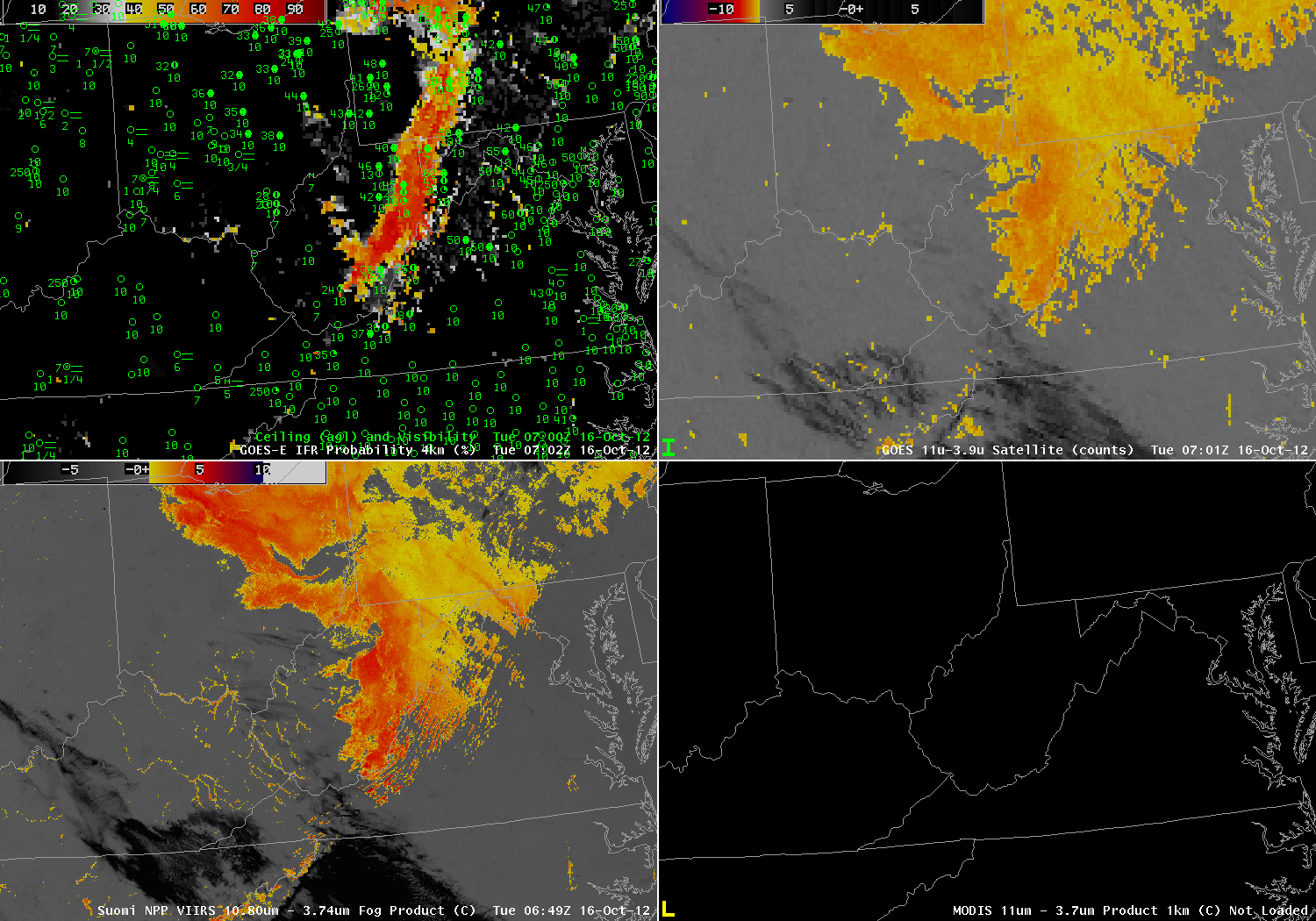
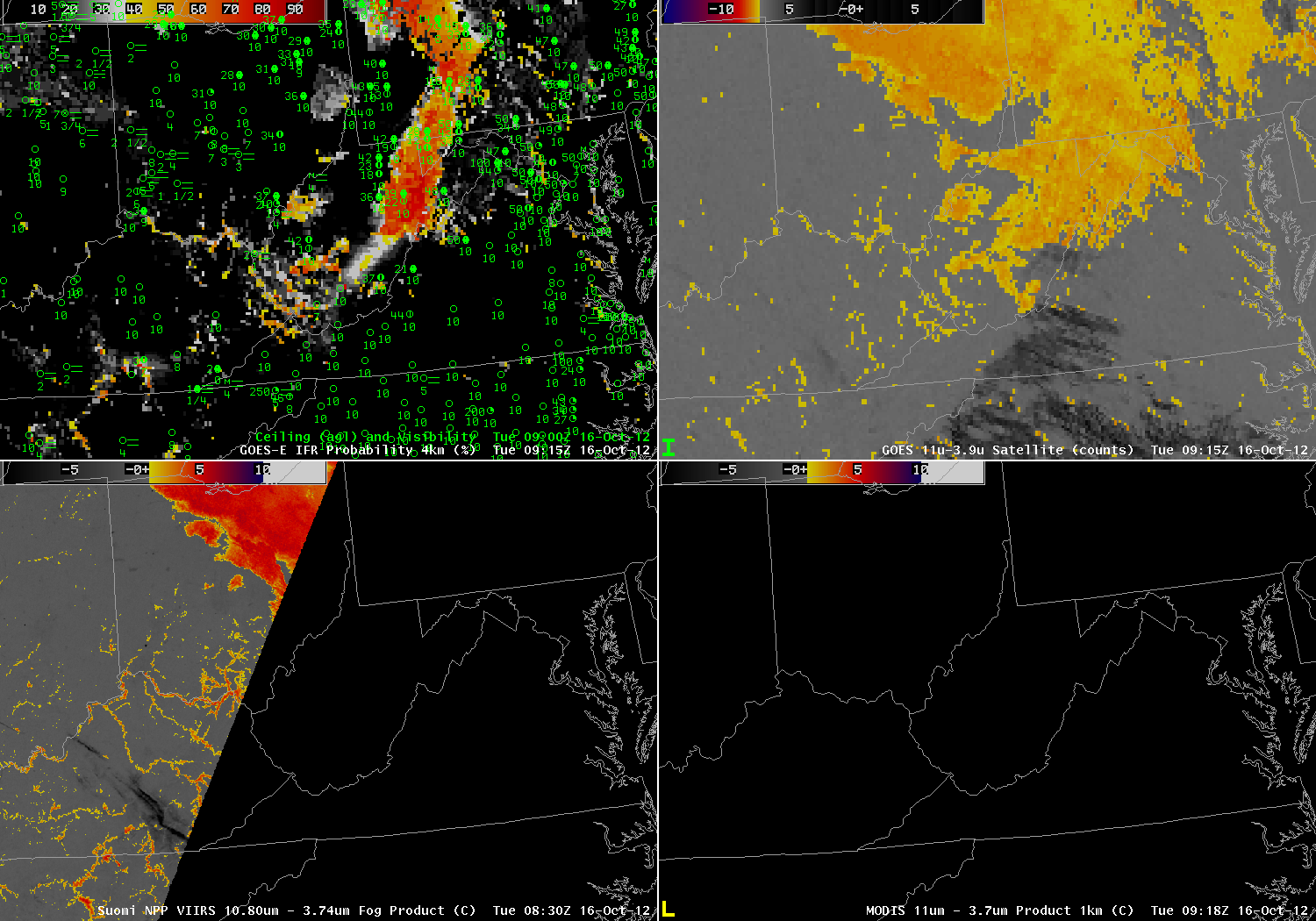
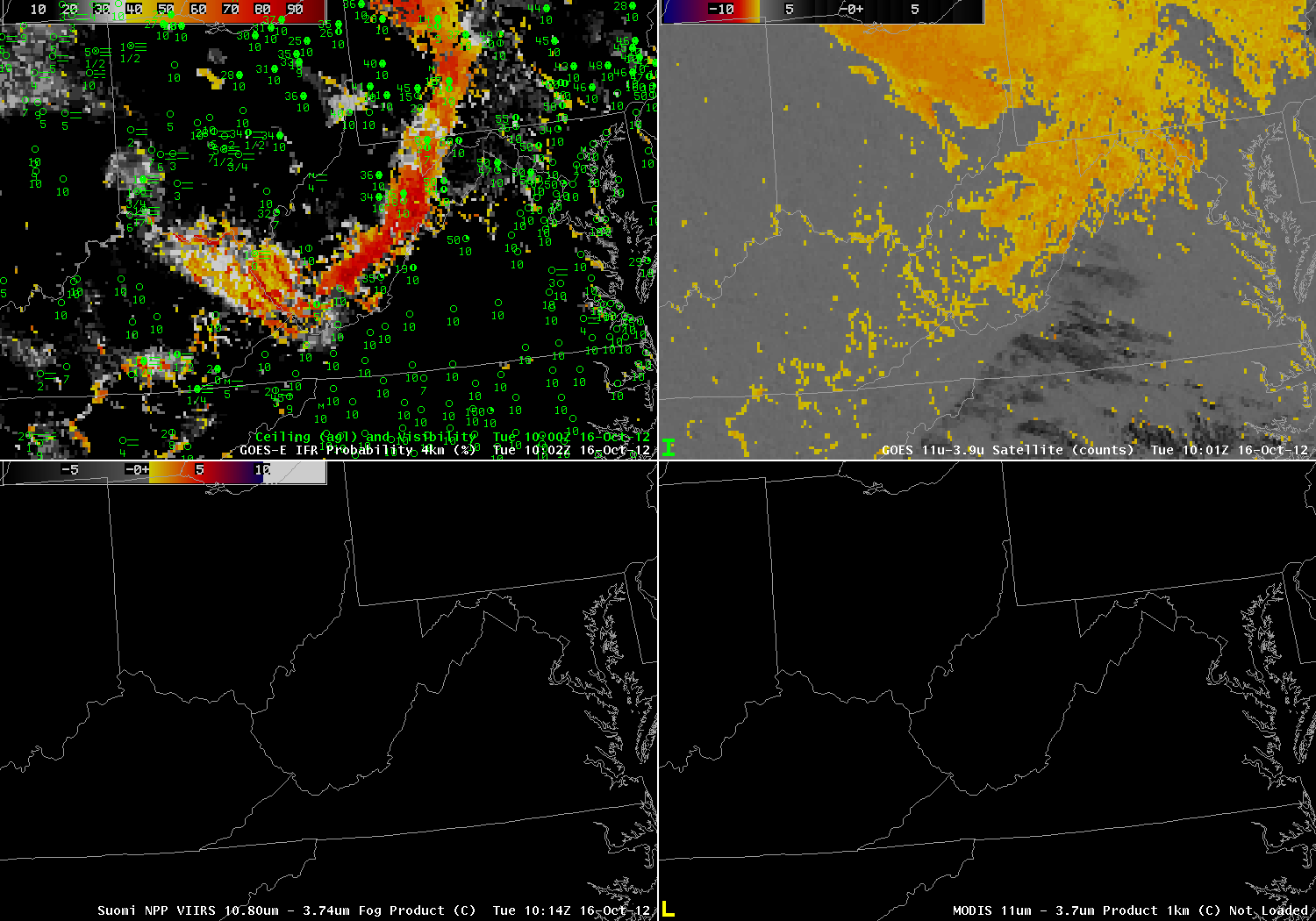
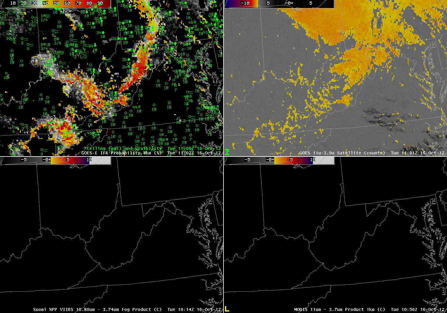
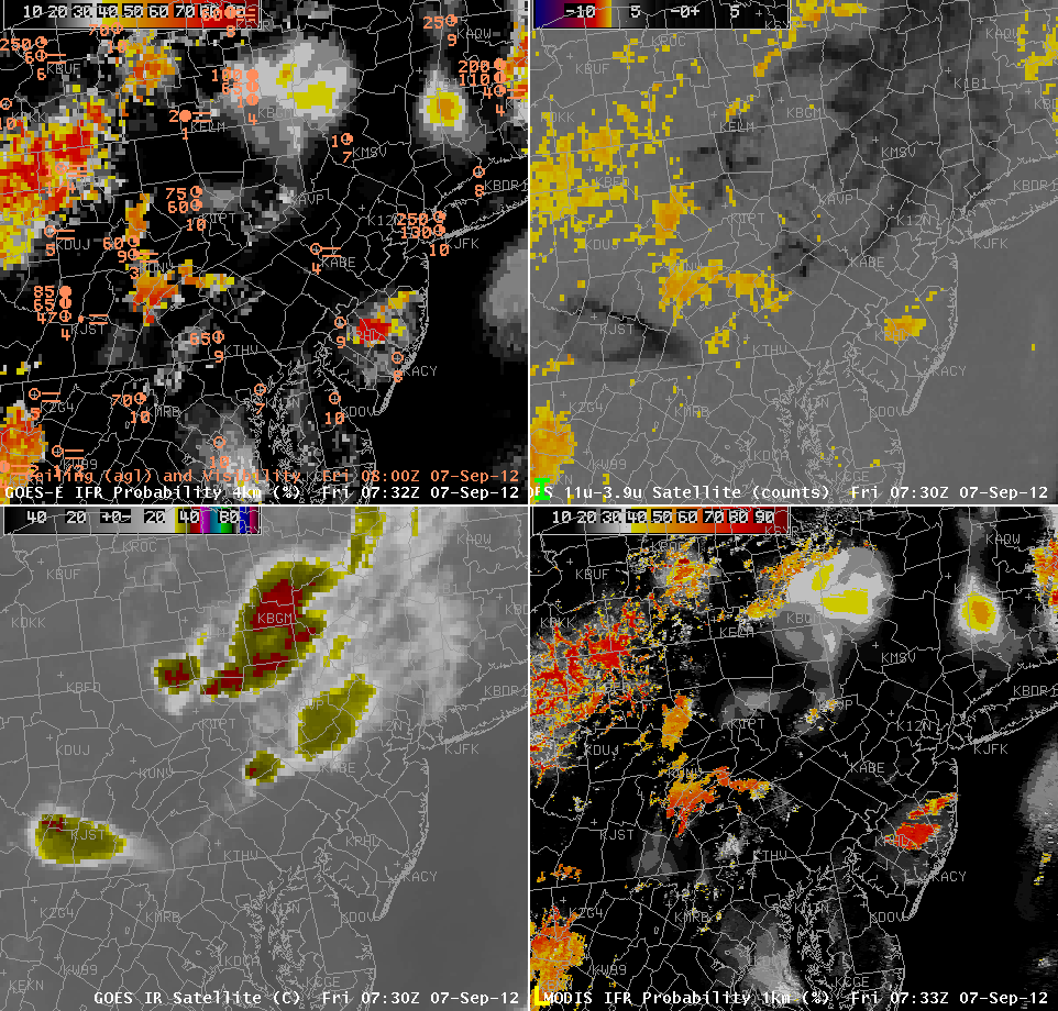
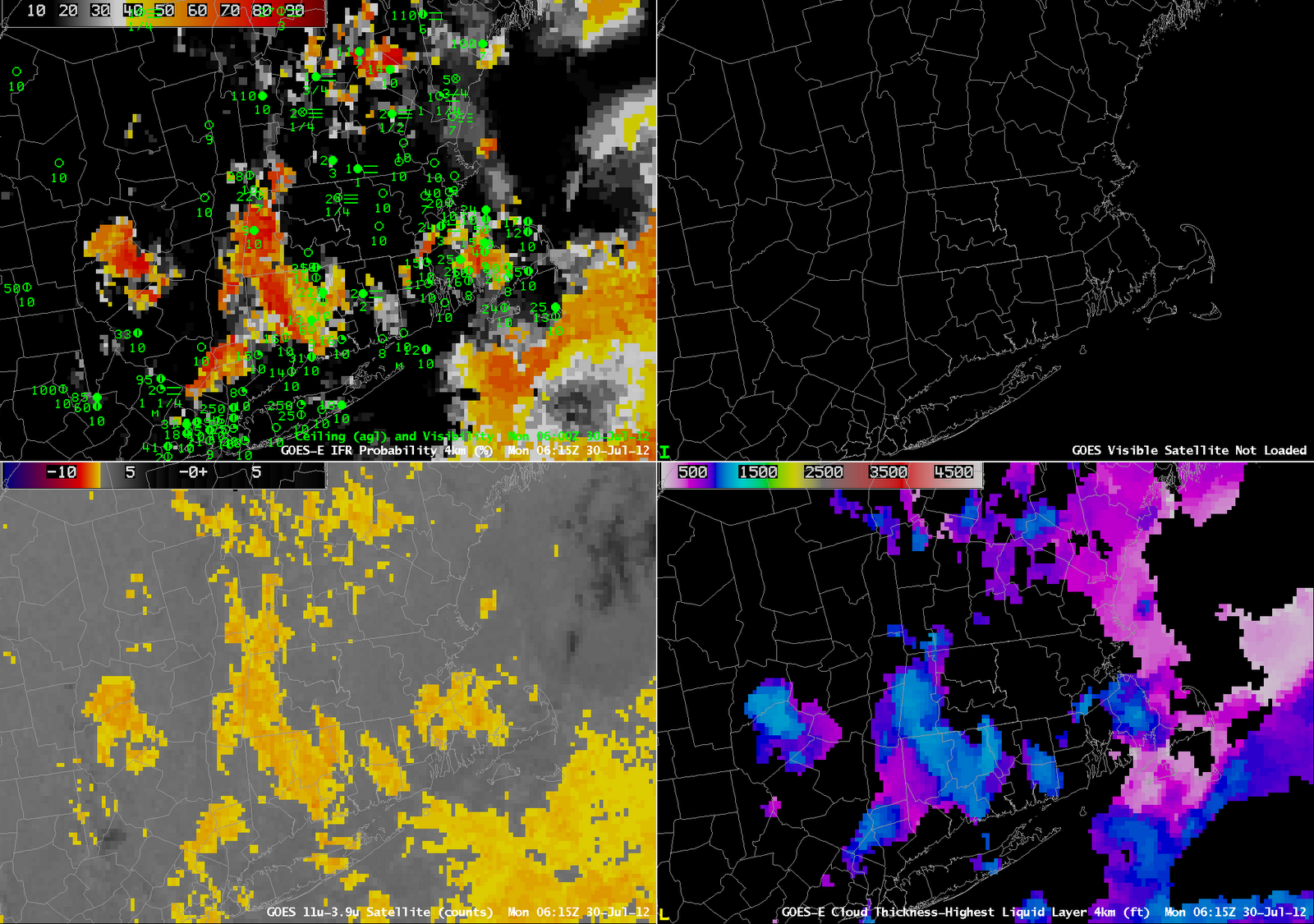
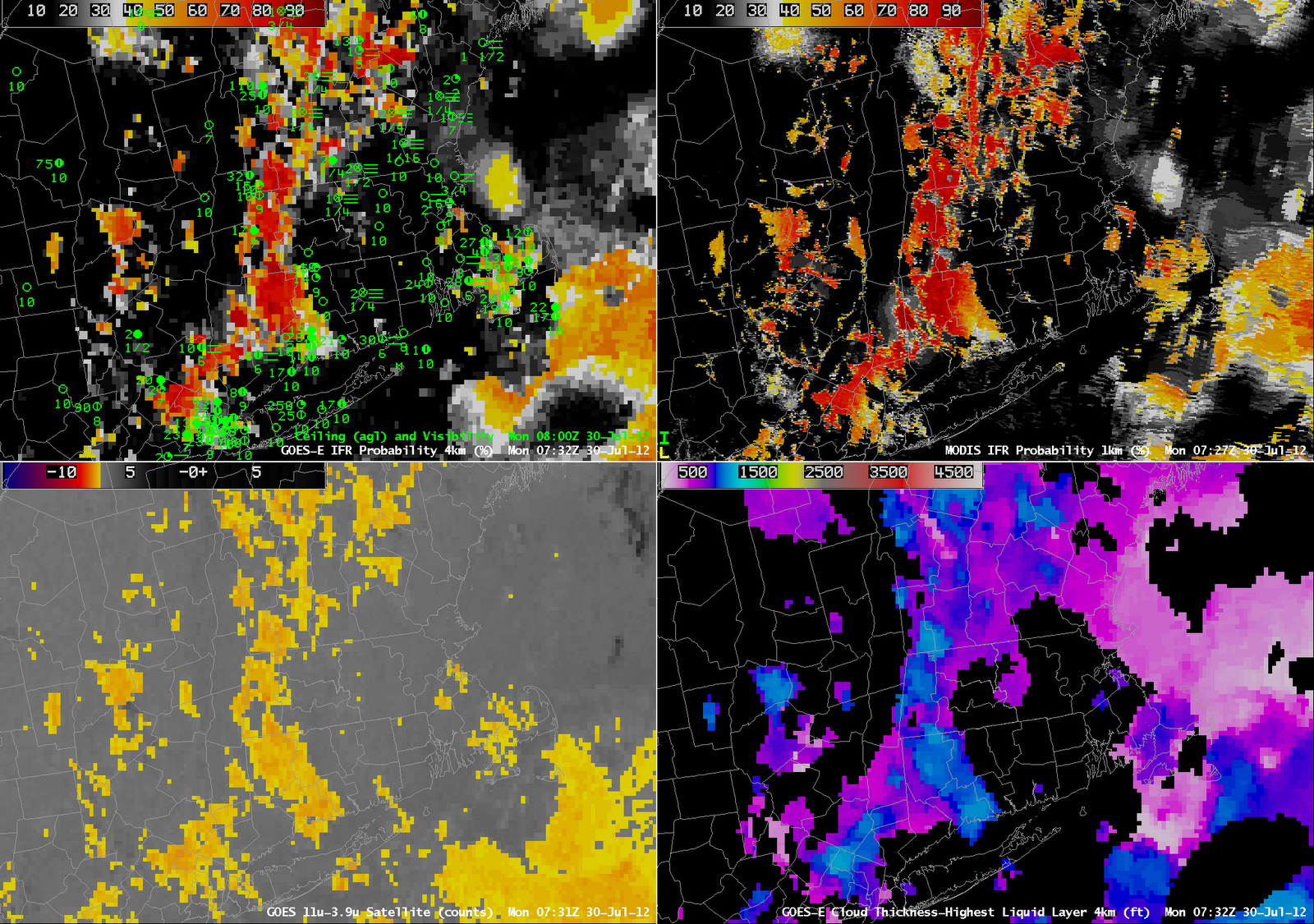
The GOES-R IFR Probability product, shown below at hourly intervals starting at 0315 UTC, shows modest probabilities of fog over the Delaware Valley, and higher probabilities over the Pine Barrens of central New Jersey, justifying the forecast mention of patchy fog.
 |
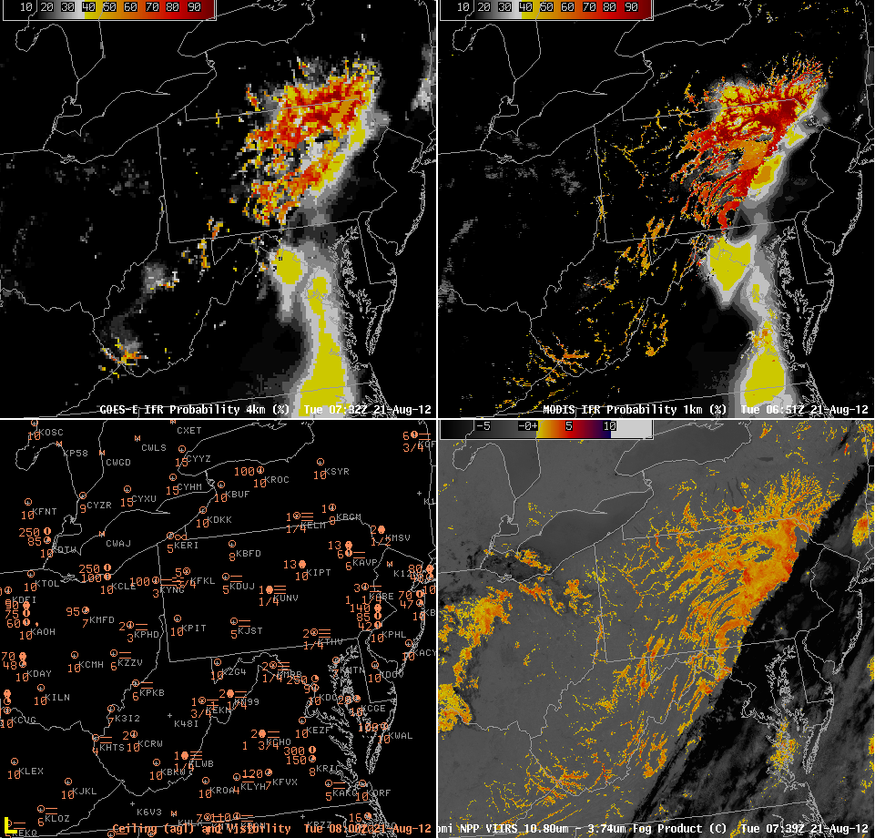
| GOES-R IFR Probabilities from GOES-East (Upper Left), Traditional Brightness Temperature Difference Product (Upper Right), enhanced window channel (Lower Left), GOES-R IFR Probabilities from MODIS (Lower left) |
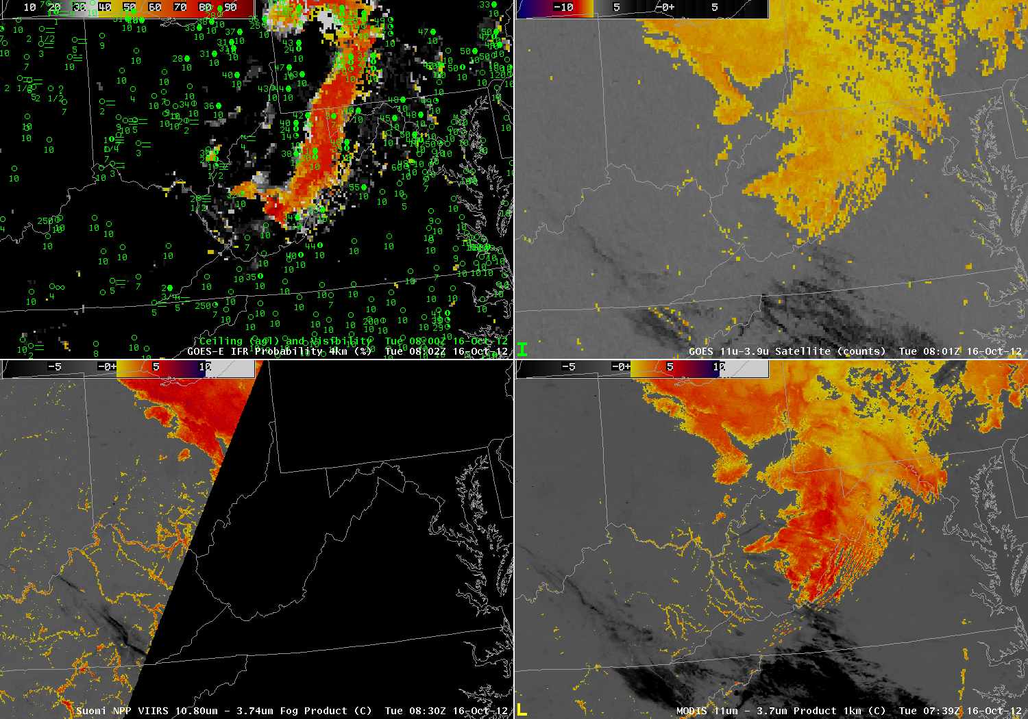
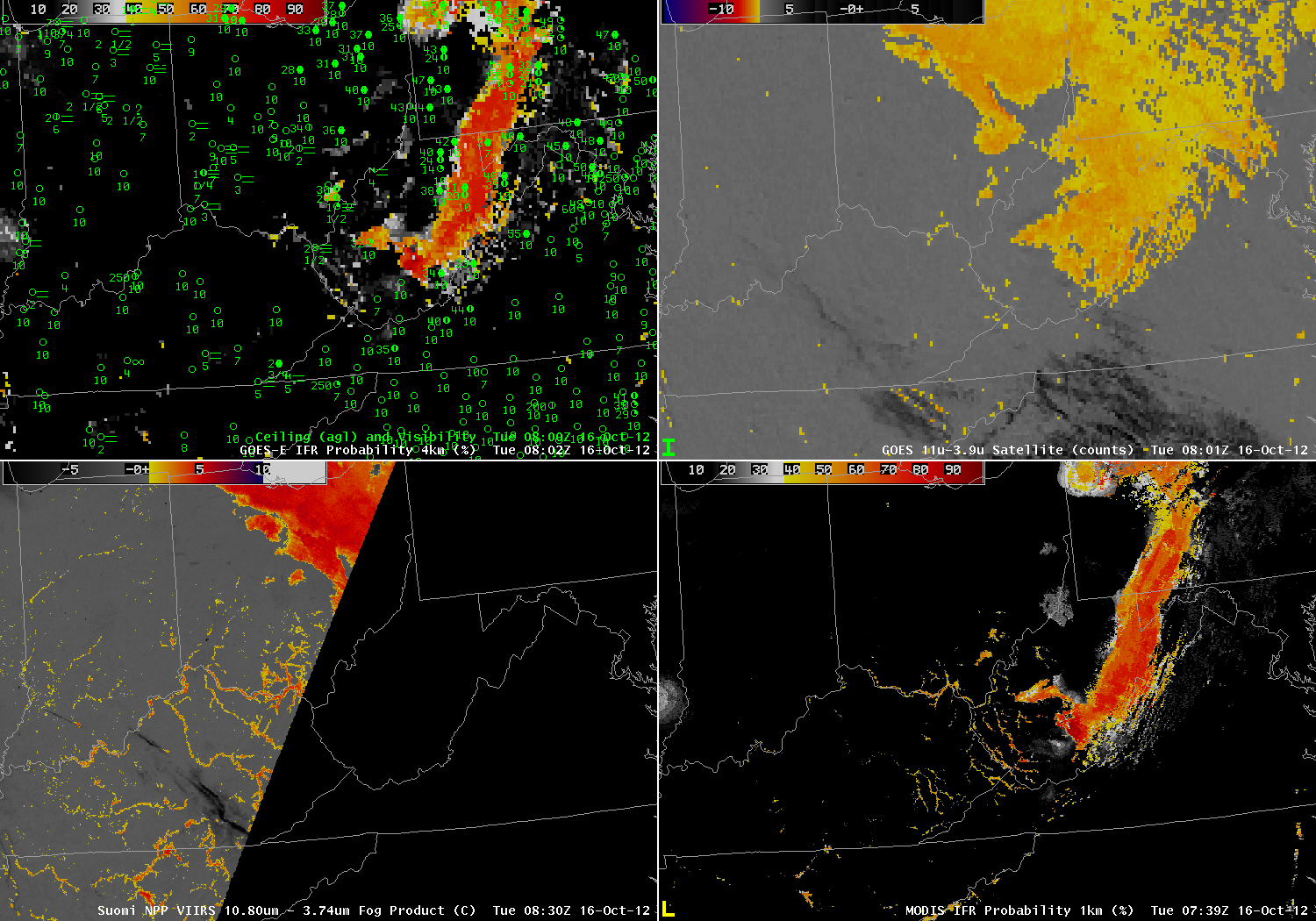
MODIS data can be used to compute IFR probabilities. One comparison scene exists at the beginning of the hourly loop, and the finer detail over the valleys of southeast Pennsylvania is evident in the 0322 UTC image. The MODIS image at 0739 UTC shows (below) similar fine-scale structures that can help a forecaster fine-tune the forecast. IFR probabilities in the MODIS images definitely jump over central New Jersey between 0322 UTC and 0733 UTC. Such a notable change is a tool for a forecaster to be alert to the possibility of fog/low stratus and IFR conditions. Several stations in central New Jersey, including McGuire Air Force base (KWRI), Belmar/Farmingdale (KBLM) and Mill Valley (KMIV) did report borderline IFR conditions between 0700 and 1000 UTC.
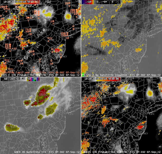 |
| GOES-R IFR Probabilities from GOES-East (Upper Left), Traditional Brightness Temperature Difference Product (Upper Right), enhanced window channel (Lower Left), GOES-R IFR Probabilities from MODIS (Lower left) from ca. 0730 UTC |