Category Archives: Mid-Atlantic

IFR Conditions over the Southeast United States

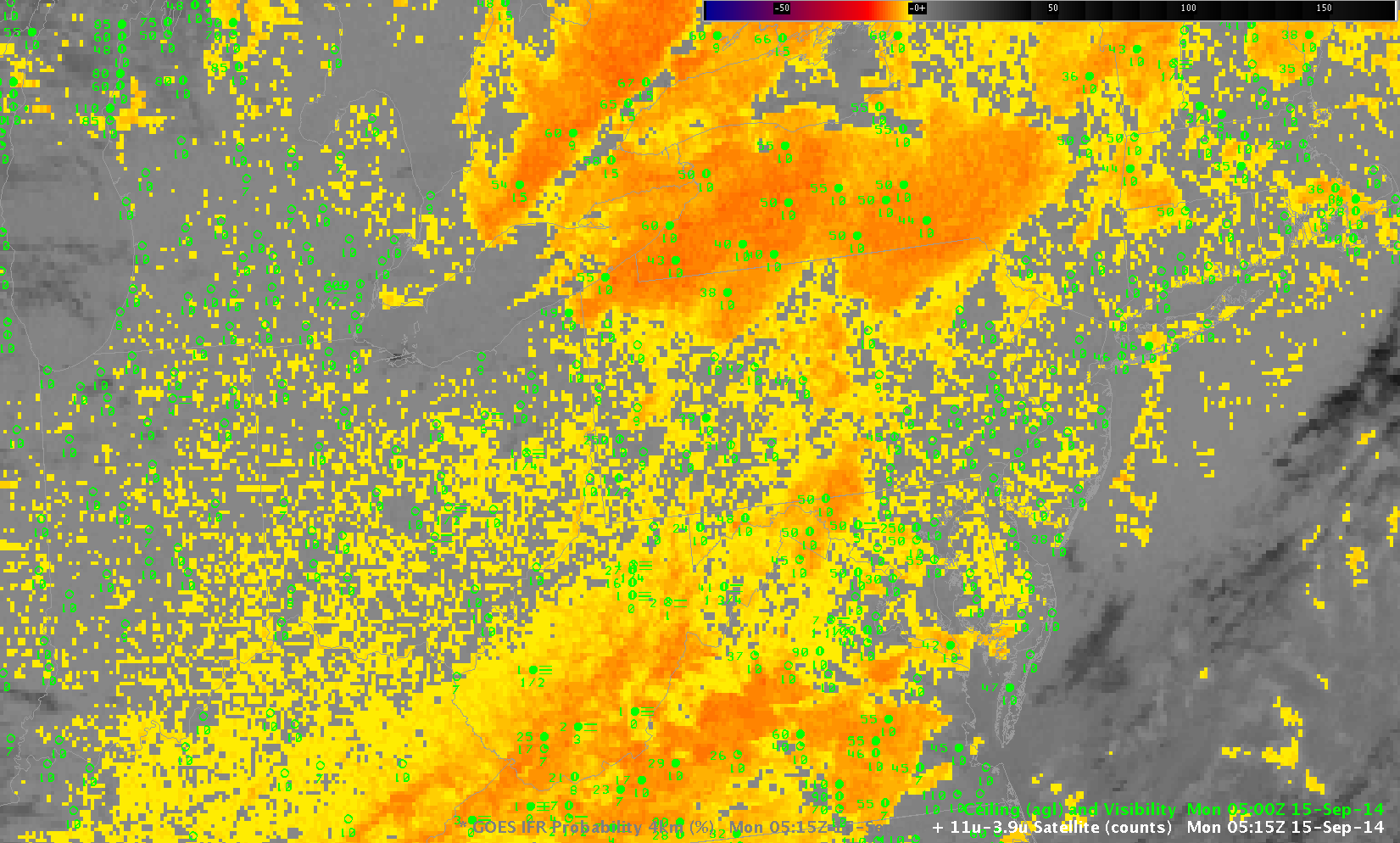
Brightness Temperature Difference Fields (10.7µm – 3.9µm) from GOES-East, hourly from 0400-1300 UTC on 2 March 2015 (Click to enlarge)

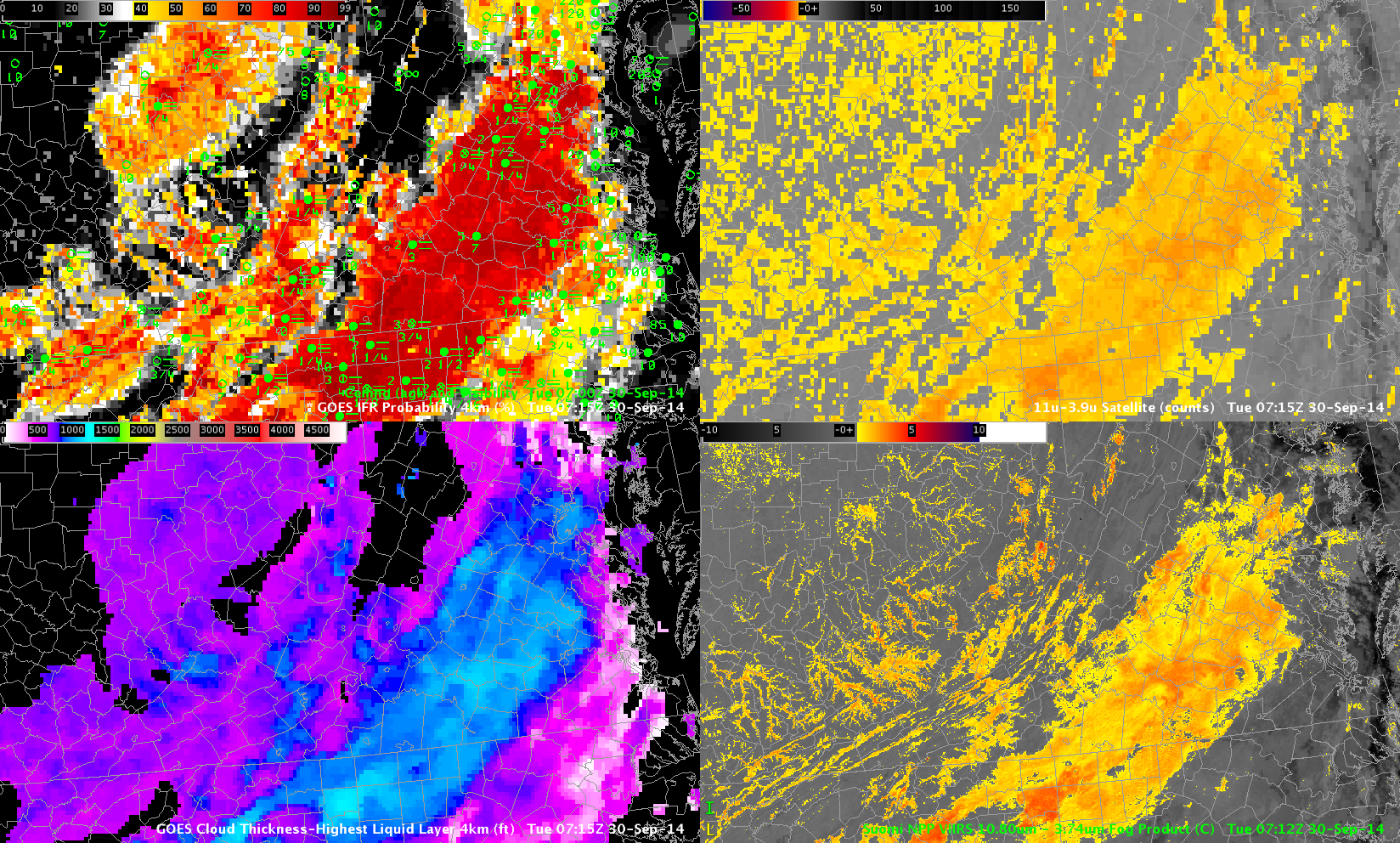
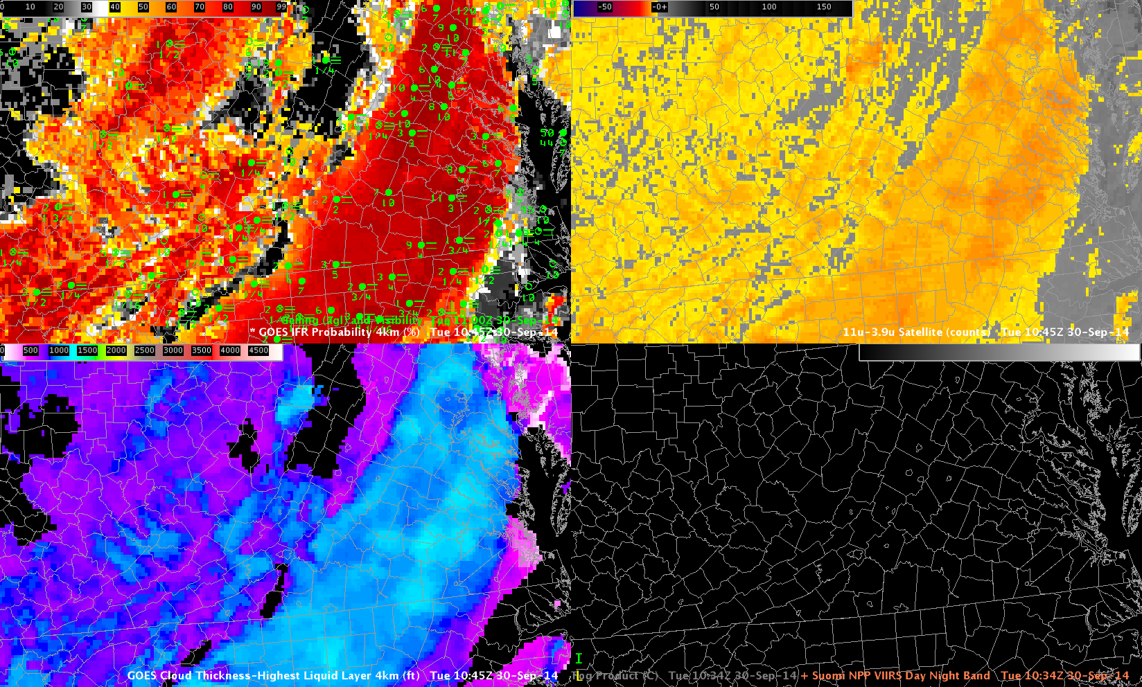
A series of frontal systems along the east coast caused multiple cloud layers and IFR conditions over much of the deep south and piedmont from Mississippi to Georgia and up through Virginia overnight on 1-2 March 2015. The animation of Brightness Temperature Difference (10.7µm – 3.9µm), above, is testimony to the difficulty in using that product as a fog detection device when multiple cloud layers are present: Many stations underneath cirrus show IFR Conditions. (Note also how the signal changes at 1300 UTC — the end of the animation — as the sun rises and increasing amounts of 3.9µm solar radiation is reflected off the clouds).

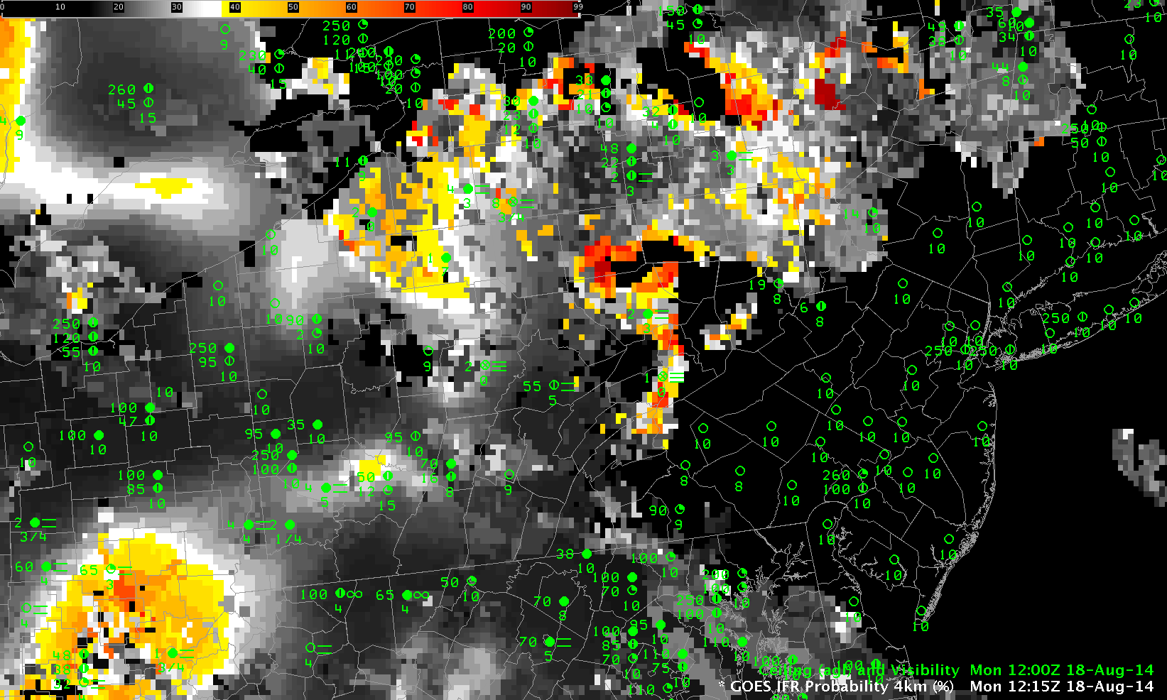
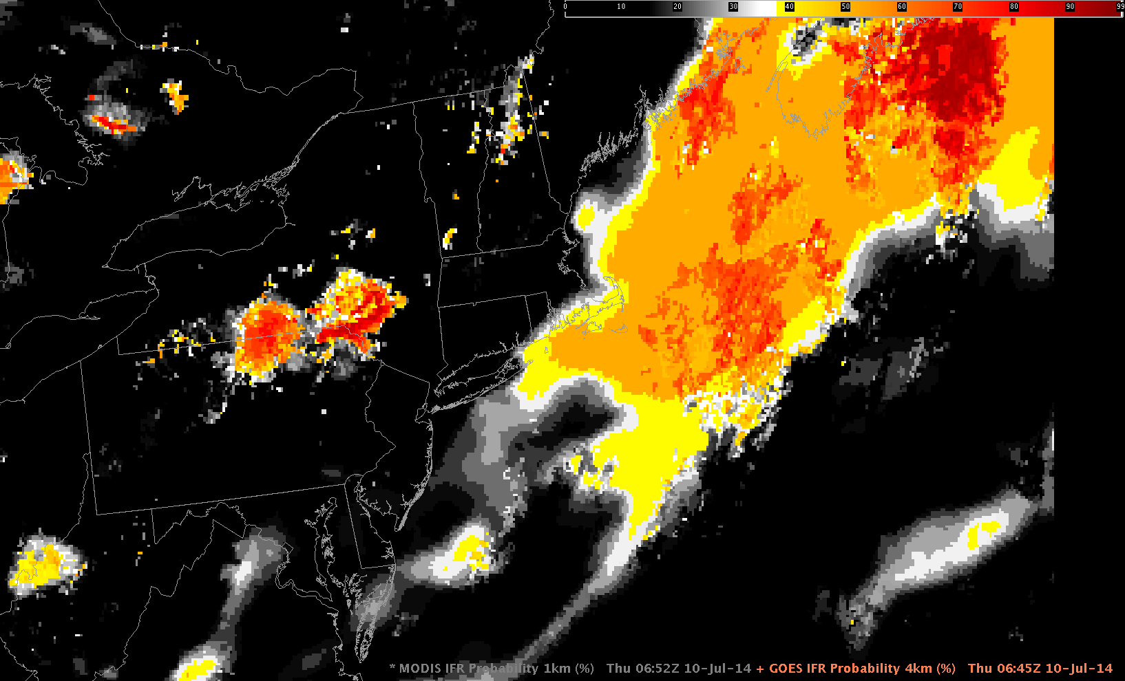
The GOES-R IFR Probability fields, below, better identify regions of reduced visibility underneath mixed cloud layers. It does this by incorporating model data (from the Rapid Refresh) into its suite of predictors. Thus, where low-level saturation is indicated under multiple cloud layers, IFR Conditions can be assumed to be occurring, and computed IFR Probabilities are large. The hourly animation of GOES-R IFR Probability, below, shows a good overlap between large IFR Probabilities and IFR (or near-IFR conditions). The flat IFR Probability field that is widespread over the Piedmont region of the Carolinas is typical of an IFR Probability field determined mostly by model output. Where high clouds break, pixelated regions develop (and IFR Probabilities increase) in the field.

GOES-R IFR Probability fields, 0400-1300 UTC on 2 March (Click to enlarge)

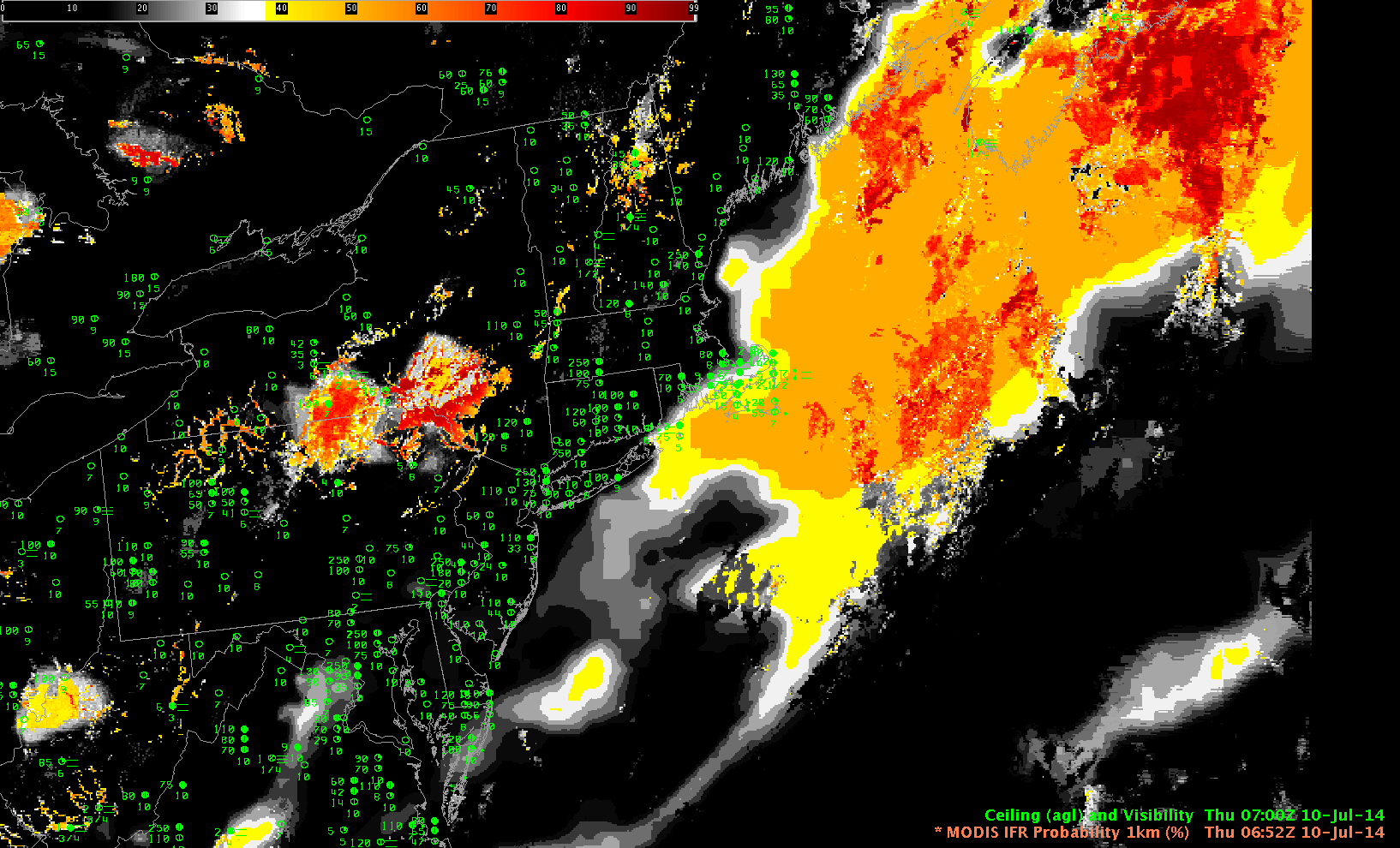
The 1215 UTC and 1300 UTC imagery in the IFR Probability animation above include a discernible nearly north-south line. (The 1215 UTC image is below). This is the terminator. To the right of that line, where IFR Probabilities are slightly larger (dark orange), daytime predictors are being used; to the left of that line, IFR Probabilities are slightly smaller (lighter orange) and nighttime predictors are being used. Why is the probability a bit larger in the daytime predictors? In part this is because visible imagery can be used to ascertain whether clouds are present. You can be a bit more confident that IFR conditions are present because clouds are present in the visible imagery.

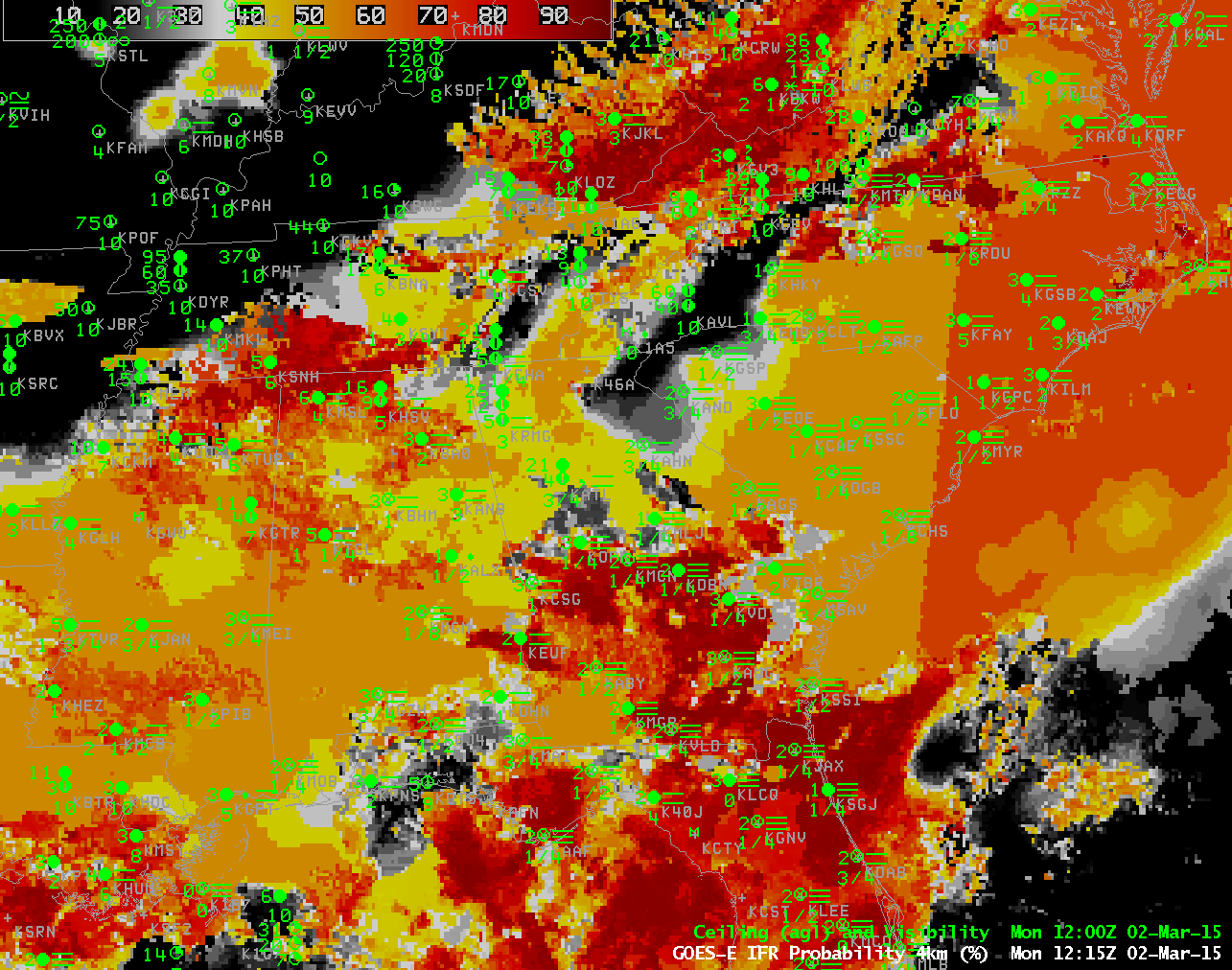
GOES-R IFR Probability fields, 1215 UTC on 2 March (Click to enlarge)

Widespread fog and low clouds along the East Coast

GOES-East Water Vapor imagery, every 2 hours, 0130 – 1330 UTC 23 December 2014 (Click to enlarge)

A slow-moving storm system is producing widespread fog and low clouds on the east coast (and in the middle of the country as well). The water vapor animation above shows the cloud cover associated with the system. Water vapor imagery such as this suggests many different cloud layers, and in such cases the IFR Probability fields (below) rely on Rapid Refresh Data to provide information because Satellite signals of low clouds cannot occur in the presence of cirrus contamination. A simple Brightness Temperature Difference product would give little information about near-surface clouds over the Southeast.

GOES-East-based GOES-R IFR Probabilities and surface-based observations of ceilings and visibilities, hourly from 0145 through 1245 UTC 23 December 2013 (Click to enlarge)

IFR Probability fields show a flat nature that occurs when satellite data cannot be used as a Predictor because of the presence of high clouds/multiple cloud layers. The Probability values are suppressed; interpretation of those values should be colored by the knowledge of the presence or absence of high clouds. In the example above, when high clouds briefly separate over central South Carolina around 0600 UTC, a region of higher IFR probability is shown. The algorithm is more confident that fog/low stratus exists because Satellite Predictors can also be used in that region. What changes is the ability of the GOES-R IFR Probability algorithm to assess the probability of IFR conditions because more predictors can be included; in the region where the high clouds part, satellite information about the low clouds can be included, and IFR Probabilities increase as a result.

More fog over South Carolina

Dense fog redeveloped over South Carolina overnight on 3-4 December 2014, and as noted in the Forecast Discussion below, its character was just a bit different than on the previous night.

000
FXUS62 KCHS 040239
AFDCHS

AREA FORECAST DISCUSSION
NATIONAL WEATHER SERVICE CHARLESTON SC
939 PM EST WED DEC 3 2014

.SYNOPSIS…
UNDER A WEAKENING WEDGE OF HIGH PRESSURE…FOG WILL PERSIST TONIGHT.
ANOTHER AREA OF HIGH PRESSURE WILL BUILD FROM THE NORTH THURSDAY THROUGH
FRIDAY. A WARM FRONT WILL THEN LIFT ACROSS THE AREA ON SATURDAY…
BEFORE A COLD FRONT MOVES THROUGH SATURDAY NIGHT. AN INLAND WEDGE
OF HIGH PRESSURE WILL BECOME ESTABLISHED SUNDAY AND MONDAY…FOLLOWED
BY THE PASSAGE OF ANOTHER COLD FRONT MONDAY NIGHT. HIGH PRESSURE
WILL THEN PREVAIL INTO THE MIDDLE OF NEXT WEEK.

.NEAR TERM /UNTIL 6 AM THURSDAY MORNING/…
WHILE THE SCENARIO IS QUITE DIFFERENT FOR FOG TONIGHT COMPARED TO
LAST NIGHT…DESPITE PLENTY OF CIRRIFORM CLOUDS /SOME OF WHICH ARE
OPAQUE/…WE ARE STILL GETTING AREAS OF FOG TO FORM. SOME OF THE
FOG IS ALREADY DENSE…ESPECIALLY IN THE CHARLESTON QUAD COUNTY
AREA AND ALONG OUR COASTAL ZONES SOUTH INTO MCINTOSH. THIS IS A
MIX OF STRATUS BUILD-DOWN AND ADVECTIVE FOG FROM OFF THE ATLANTIC.
SO WE LOOK FOR A FURTHER EXPANSION OF THE FOG INLAND TO THE WEST
OF I-95 THROUGH THE NIGHT. DENSE FOG ADVISORIES WILL THEREFORE
REMAIN IN EFFECT.

GOES-based GOES-R IFR Probabilities, hourly from 2315 UTC 3 December through 1015 UTC on 4 December as well as observations of ceilings (AGL) and visibilities (Click to enlarge)

GOES-R IFR Probabilities, above, (click here for an animation with a faster dwell rate) once again capably outlined the region of IFR conditions over South Carolina. Probabilities are lower when Satellite data cannot be used as a predictor, as when cirrus clouds prevent the satellite from viewing water-based clouds closer to the surface. In such cases when only Rapid Refresh model data can be used as Fog Predictors, the fields take on a flatter, less pixelated character as above. There are a few regions where breaks in the cirrus cloud allow Satellite predictors to be incorporated in the IFR Probability fields, for example along the South Carolina coast at 0600 UTC. When high clouds are present, interpret the magnitude of the IFR Probability in a different way than when high clouds are absent. An IFR Probability of 55% in a region of cirrus clouds has a different meaning than an IFR Probability of 55% in a region of only low clouds.

Because of Cirrus clouds, the brightness temperature difference fields gave almost no information about the presence of low clouds. See the animation below (a loop with a faster dwell rate is here).

GOES-13 Brightness Temperature Difference Fields (10.7µm – 3.9µm), hourly from 2315 UTC 3 December through 1015 UTC on 4 December, as well as observations of ceilings (AGL) and visibilities (Click to enlarge)

Dense Fog over South Carolina

Dense fog devloped over South Carolina overnight, in an event that was well-anticipated: From the Charleston, SC, National Weather Service Office AFD (emphasis added):

AREA FORECAST DISCUSSION
NATIONAL WEATHER SERVICE CHARLESTON SC
648 PM EST TUE DEC 2 2014

.SYNOPSIS…
WEAK HIGH PRESSURE WILL PERSIST THROUGH WEDNESDAY. A COLD FRONT
WILL ADVANCE SOUTH THROUGH THE AREA THURSDAY…THEN HIGH PRESSURE
WILL BUILD FROM THE NORTH AND WILL PREVAIL THROUGH FRIDAY. LOW
PRESSURE WILL TRACK THROUGH OR JUST NORTH OF THE REGION SATURDAY…
FOLLOWED BY COLD FRONTS SATURDAY NIGHT AND AGAIN LATE MONDAY.

.NEAR TERM /UNTIL 6 AM WEDNESDAY MORNING/…
A FEW LINGERING STRAY SHOWERS WEST OF I-95 WILL DISSIPATE THIS
EVENING WITH THE ONSET OF NOCTURNAL COOLING AND STABILIZATION.

OUR MAIN FOCUS FOR TONIGHT IS IN REGARDS TO FOG AND THE BUILD DOWN
OF STRATUS…SOME OF WHICH COULD BE DENSE. THE HIGH PRESSURE WEDGE
WILL REMAIN ANCHORED OVER THE INLAND PARTS OF THE SE AS IT
PROGRESSES A LITTLE SOUTHWARD THROUGH THE NIGHT…WITH A WEAK
COASTAL TROUGH OFFSHORE. A STRENGTHENING NOCTURNAL INVERSION WILL
DEVELOP AND TRAP ABUNDANT MOISTURE WITHIN THE PLANETARY BOUNDARY
LAYER UNDERNEATH. THIS WILL LEAD TO THE DEVELOPMENT AND SPREADING
OUT OF FOG AND STRATUS ENCOMPASSING MOST IF NOT ALL OF THE CWFA
DURING THE LATE NIGHT HOURS. BUT ALREADY WE/RE SEEING A FOG BANK
WITH IT/S ORIGINS NORTH OF THE SANTEE RIVER THIS AFTERNOON IS
PROGRESSING SOUTH/SW AND STARTING TO SPREAD A LITTLE INLAND. THIS
IS CLEARLY DEPICTED BY THE 11-3.9 MICRON SATELLITE IMAGERY AS WELL
AS COASTAL METAR SITES. THE COMBINATION OF THE MARINE INDUCED FOG
AND STRATUS WILL COMBINE WITH RADIATION FOG THAT FORMS OVER INLAND
SECTIONS TO RESULT IN AREAS OF FOG ACROSS THE FORECAST ZONES. THE
WORST CONDITIONS WILL BE OVER CHARLESTON COUNTY THIS
EVENING…SPREADING INTO OTHER COASTAL SC ZONES LATER THIS EVENING
AND INTO THE GA COASTAL ZONES BY MIDNIGHT OR SO. INLAND THE BULK
OF THE GREATER FOG/STRATUS COVERAGE WILL WAIT UNTIL WE REACH OUR
CROSS-OVER TEMPS BY 2-3 AM. DENSE FOG ADVISORIES ARE CERTAINLY
POSSIBLE. ANY NEGATING FACTORS AGAINST THE WIDESPREAD DENSE FOG
WOULD BE THE RELATIVELY WARM GROUNDS. BUT GIVEN FOG STABILITY
INDICES IN THE TEENS AND LOWER 20S…MOST PLACES REACHING THEIR
CROSS-OVER TEMPS OF 55-60 AND SOME MARINE FOG WE/D LEAN MORE
TOWARD DENSE FOG BECOMING A CONCERN…THAN NOT.

GOES-based GOES-R IFR Probabilities, hourly from 2215 UTC 2 December through 1315 UTC on 3 December as well as observations of ceilings (AGL) and visibilities (Click to enlarge)

The GOES-R IFR Probability fields, shown at hourly intervals above, nicely capture the spread of the extensive fog as the expanding marine fog bank joins up with the developing radiation fog over northwestern South Carolina. (A loop with a shorter dwell rate is here). GOES-13 Brightness Temperature Difference Fields are shown below. (A loop with a shorter dwell rate is here). Brightness Temperature Difference is the traditional method of detecting fog and low stratus, and it is referenced in the AFD above. However, the method cannot operate in regions with high cirrus (such as over Tennessee and northwest South Carolina after 0900 UTC); the brightness temperature difference signal flips sign as the sun rises (as at 1315 UTC in the animation below); the method cannot distinguish between elevated stratus and visibility-restricting fog.

GOES-13 Brightness Temperature Difference Fields (10.7µm – 3.9µm), hourly from 2215 UTC 2 December through 1315 UTC on 3 December, as well as observations of ceilings (AGL) and visibilities (Click to enlarge)

In comparing the two animations, note how the Brightness Temperature Difference field, for example, has strong returns around 0215-0315 UTC over central South Carolina in regions where widespread IFR conditions do not yet exist. In these regions, the Rapid Refresh model data used as a predictor in the GOES-R IFR Probability is not yet showing saturation, so IFR Probabilities aren’t quite so high as they are along the coast. (Click here for a toggle between the GOES-R IFR Probability and the Brightness Temperature Difference fields at 0215 UTC; a toggle at 0315 UTC is here). Note also in the toggles how the IFR Probability fields have little signal over Georgia despite the Brightness Temperature Difference field signal. This demonstrates the power of using fused data products: both the satellite and the model signal must be in accord for very high probabilities to occur.

MODIS vs. GOES-based IFR Probabilities

MODIS-based and GOES-based IFR Probability fields at ~0300 UTC on 03 October 2014 (click to enlarge)

A great benefit of a polar-orbiting satellite, such as Terra, or Aqua, or Suomi NPP, is that they provide very high-resolution imagery. The toggle above shows the early development of overnight fog over the mountainous terrain of Pennsylvania. The MODIS IFR Probability resolves with clarity the small river valleys of north-central Pennsylvania. Both MODIS and GOES suggest higher probabilities over the elevated terrain (the Laurel Highlands near Johnstown and regions around Bradford). A later overpass, below, just after 0700 UTC, shows the expansion of the regions of high probability has occurred in both MODIS and GOES-based products, but the MODIS-based product continues better to resolve the river valleys, such that Probabilities are higher over River Valleys (over the Pine Creek basin of north-central Pennsylvania, for example).

MODIS-based and GOES-based IFR Probability fields at ~0700 UTC on 03 October 2014 (click to enlarge)

Suomi NPP also provides high-resolution imagery, and sometimes orbital geometry allows two consecutive orbits – about 90 minutes apart — to view the same region, as below over Pennsylvania. This also shows the general increase in fog/low stratus over the eastern two-thirds of the state. (IFR Probability algorithms do not yet include Suomi NPP data).

Suomi NPP Brightness Temperature Difference (11.35µm – 3.74µm) Fields at 0617 and 0756 UTC 03 October 2014 (click to enlarge)

Polar orbiters lack good routine temporal resolution, a shortcoming that can be a significant drawback. For example, none of the satellites are overhead just before sunrise, a time when the start of the morning commute might demand information. For that, GOES data (with its 15-minute temporal resolution) is essential. The 1145 UTC image, below, shows IFR Probabilities over the region at that time, and GOES data are routinely used to monitor the evolution of IFR Probability fields over the course of the night.

GOES-based IFR Probability fields at 1145 UTC on 03 October 2014 (click to enlarge)

Fog over the Piedmont of Virginia

GOES-R IFR Probabilities (Upper Left), GOES-R Cloud Thickness (Lower Left), Brightness Temperature Differences from GOES-13 (Top Right, 10.8 µm – 3.9 µm) and from Suomi-NPP (Bottom Right, 11.35 µm -3.74 µm , all at 0715 UTC 30 September (Click to enlarge)

Radiation fog developed over the Piedmont of Virgina on the morning of 30 September in a region with little pressure gradient. The image above, from 0715 UTC, shows IFR Probability to be very high (from 85-95%) over the Virginia Piedmont. Numerous stations in the region were reporting IFR visibilities and ceilings. Brightness Temperature Difference products are also highlighting the region (Note the advantage in the Suomi NPP Brightness Temperature Difference field that ably captures fine detail related to Ridge/Valley topography over the Appalachians); the advantage of IFR Probability fields is that it includes surface information so that someone using the field can be more certain that the stratus detected by the satellite is in contact with the ground as fog. The animation below shows the evolution of the fields from 0200 through 0700 UTC.

As above, but with Suomi NPP Day/Night band in lower Right. Hourly imagery from 0200 through 0700 UTC on 30 September 2014 (Click to enlarge)

GOES-R Cloud Thickness (the thickness of the highest water-based cloud) can be used to estimate when fog/low clouds will burn off. The estimate is most accurate for strict radiation fog. GOES-R Cloud Thickness is only computed for water-based clouds during non-twilight times (in other words, it is not computed in the hours surrounding twilight at both sunrise and sunset). The last value of Cloud Thickness before morning twilight (shown below) can be used in concert with this scatterplot to guess when clouds might dissipate. Values over eastern Virginia, near Richmond, exceeding 1100 feet, correspond to a dissipation time 4+ hours after 1100 UTC, or at 1500 UTC. In this case, that value was an underestimate.

As above, but for 1100 UTC 30 September 2014

GOES-13 Visible imagery, hourly between 1215 and 1715 UTC 30 September 2014 (Click to enlarge)

Stratus and Fog over the northeast and mid-Atlantic States

GOES-13 Color-Enhanced Brightness Tempreature Difference Fields (10.7 µm – 3.9 µm), hourly from 0200 through 1100 UTC, 15 September 2014 (Click to enlarge)

Brightness Temperature Difference Fields from GOES-13 show large regions over Pennsylvania and surrounding states during the early morning hours of September 15th. (Note that the image at 0515 UTC, not in the loop above, shows the effect of stray light). If you look at the ceilings and visibilities in the imagery above, you will note that many regions where stratus/fog are indicated by the brightness temperature difference field (over upstate NY, for example), do not in fact show anything near IFR conditions. Always recall that the satellite is seeing the top of the cloud deck; whether or not that cloud extends to the surface is beyond the capability of present satellite systems. (You can infer it sometimes, of course, especially if the signal is confined to a narrow river valley, as occurs in the animation above: The Ohio River along the northern panhandle of West Virginia shows up very well).

GOES-13 IFR Probability Fields, hourly from 0200 through 1100 UTC, 15 September 2014 (Click to enlarge)

IFR Probability fields for the same time do a better job of highlighting only where reduced ceilings and visibilities are present. For example, the region of stratus over upstate New York is screened out, as well as the region over southern and southeastern Virginia. Probabilities are also quite high over the Ohio River Valley, where river fog is likely occurring. Note that IFR Probabilities over southwestern Indiana at the end of the animation have the characteristic look (a flat field) associated with IFR Probabilities created without the benefit of satellite data.

MODIS data were able to provide a a high-resolution image of this scene in the middle of the night. As with GOES, MODIS identified the large region of stratus over upstate New York and over southeastern Virginia, and the IFR Probabilities correctly screened out those stratus clouds. River Valleys show up distinctly along the Ohio River downriver from Pennsylvania; smaller IFR Probabilities surround the rivers. Sometimes MODIS data can give an early alert to the development of fog; in the present case, when MODIS overflew the region, fog development was at sufficiently large a scale that GOES-13 could also detect it.

MODIS Color-Enhanced Brightness Tempreature Difference Fields (11 µm – 3.9 µm) and IFR Probability Fields at 0722 UTC 15 September 2014 (Click to enlarge)

Suomi NPP data also viewed the developing river fogs, both in the day/night band, and in the brightness temperature difference (11.35 µm – 3.74 µm), below. At present, IFR Probabilities are not computed from Suomi NPP satellite data.

Suomi NPP Color-Enhanced Brightness Tempreature Difference Fields (11.35 µm – 3.74 µm) and Day Night band visible imagery at 0653 UTC 15 September 2014 (Click to enlarge)

Fog over Pennsylvania

GOES-R IFR Probabilities computed from GOES-13 data, hourly from 0500 through 1300 UTC 18 August 2014

River valley fog developed over Pennsylvania during the early morning hours of 18 August 2014, and the case is a good test of the GOES-R IFR Probability fields. IFR Probabilities are low at 0500 UTC (1 AM local time) and subsequently increase rapidly. In this case, the fields may be overpredicting where fog is present, as visible imagery just after sunrise suggest it was confined mostly to river valleys. In the animation above, the areal extent of the IFR Probabilities drops between 1100 UTC and 1215 UTC as the sun rises (the terminator is apparent in the 1100 UTC image, running from western Maryland north-northwestward to extreme western New York) and visible imagery can be used to more effectively cloud-clear the fields. A toggle between these two times is below. In this case, it is important to understand the geography underneath the IFR Probability field to hone the forecast.

GOES-R IFR Probabilities computed from GOES-13 data, at 1100 and 1215 UTC 18 August 2014

GOES-East Brightness Temperature Difference Fields (10.7µm – 3.9µm), hourly, from 0500-1100 UTC 18 August 2014

The Brightness Temperature Difference field, above, is the heritage method of detecting low stratus and inferring the presence of fog. Interpretation is complicated because high clouds (initially present over the southwestern portion of the scene, and moving eastward) prevent the satellite from viewing low clouds. In addition, as the sun rises (at the end of the animation, at 1100 UTC), solar radiation changes the character of the the brightness temperature difference field.

Data from the MODIS on board both Terra and Aqua can also be used to create both brightness temperature difference fields and IFR Probability fields. The toggle below, using ~0700 UTC data from GOES and from MODIS, shows the distinct advantage present in the MODIS field’s superior spatial resolution (1-km at sub-satellite point vs. 4-km at the sub-satellite point for GOES). River valleys are more evident in the MODIS data, by far, than in the GOES data.

GOES-R IFR Probabilities computed from GOES-13 data and from MODIS data, at 0700 UTC 18 August 2014

The Day-Night band on Suomi NPP at 0718 UTC showed that the densest fog was largely confined to river valleys.

Suomi NPP Day/Night Band, 0718 UTC on 18 August 2014

An animation of the fog burning off from GOES-14 (in special 1-minute SRSO-R scanning operations) is available here. It’s also on YouTube.

Fog and low stratus over the North Carolina piedmont

Hourly imagery of GOES-R IFR Probabilities over North Carolina, 0500-1400 UTC 23 July 2014, including surface observations of ceilings and visibilities

Low ceilings and reduced visibilities developed along the North Carolina piedmont during the morning of July 23rd. GOES-R IFR Probabilities showed the stripe of low ceilings/reduced visibilities extending northeast to southwest along the Piedmont. Observed IFR and near-IFR conditions roughly correlate with higher probabilities in the field displayed. Note that probabilities increase between 1100 and 1200 UTC, when the Sun rises and different predictors are used to compute the fields.

In contrast, the brightness temperature difference field (below) does not have a strong signal, it would be difficult to use the fields to predict where fog/low stratus would be.

GOES-R IFR Probabilities allow a better description of where fog/low stratus exists because of the use of Rapid Refresh data as a predictor of fog. In cases where the satellite signal is not strong, such as this one, saturation information from the model adds critical information.

Hourly imagery of GOES-13 Brightness Temperature Differences (10.7 µm – 3.9 µm) over North Carolina, 0500-1400 UTC 23 July 2014, including surface observations of ceilings and visibilities

Distinguishing between stratus and fog over Pennsylvania

Suomi NPP 11.35 µm Infrared Imagery at 0609 and 0752 UTC, 10 July 2014 (Click to enlarge)

The orbital geometry of Suomi NPP allowed two high-resolution images of Pennsyvlania early in the morning of the 10th of July 2014. Can you tell from the imagery above if there is fog/stratus in the river valleys of Pennsyvlania? Are the relatively cool clouds from Pittsburgh northeastward towards Elmira, NY obstructing visibilities? Based on the IR (11.35 µm for Suomi NPP) imagery alone, above, that is a difficult question to answer. Historically, the brightness temperature difference between the longwave IR (11.35 µm) and the shortwave IR (3.74 µm) has been used to indentify water-based clouds. Imagery from Suomi NPP, below, highlights where water-based clouds (like stratus) exist. If the clouds are the same temperature as the surrounding land (likely the case for river fog), a single 11.35-µm image is of little help in identifying the clouds.

Suomi NPP 11.35 – 3.74 µm Brightness Temperature Difference at 0609 and 0752 UTC, 10 July 2014 (Click to enlarge)

The Day-Night band can also highlight where clouds exist, because lunar illumination reflects well off clouds. A 3/4-full moon ably illuminates the scene at 0609 UTC, but that moon has set at 0747 UTC and the Clouds are harder to see.

Suomi NPP Day/Night Band at 0609 and 0752 UTC, 10 July 2014 (Click to enlarge)

Both the Day/Night band and the Brightness Temperature Difference Fields (and any Infrared image) gives information about the top of the cloud. Fog existence is difficult to discern only from satellite data because the bottom of the cloud is not sampled. This is why a fused product (such as IFR Probability) that includes surface information (in the case of IFR Probability from the Rapid Refresh Model) is desirable. MODIS data can be used to compute IFR Probability, and a MODIS-carrying Aqua pass occurred in between the two Suomi NPP Passes shown above.

MODIS 11 – 3.9 µm Brightness Temperature Difference and IFR Probability at 0652 UTC, 10 July 2014 (Click to enlarge)

In the two images above, note how the IFR Probability Fields de-emphasize the low cloud areas that stretch northeastward from Pittsburgh towards Elmira. This is likely mid-level stratus. River Fog over northeast Pennsylvania is highlighted in the IFR Probability fields (and in the brightness temperature difference field). This image, which shows the GOES-based IFR Probability field at 0645 UTC, highlights the power of MODIS’ superior spatial resolution in the early detection of small-scale fog. The large region of reduced visibility around Elmira NY (meager surface observations suggest this large region of fog verified) appears in both MODIS- and GOES-based IFR Probability fields. Only the MODIS-based IFR Probability field, however, has a distinct river-valley signal over northeast Pennsylvania.

MODIS and GOES IFR Probability both suggest IFR conditions may be occurring over the Atlantic Ocean. The brightness temperature difference field shows no low cloud signal there because of a cirrus shield. IFR Probability gives a signal of fog here based on information from the Rapid Refresh.

GOES-R Fog Product Examples

Fog detection fusing GOES, Terra/Aqua or Suomi/NPP Satellite data with Model output