Category Archives: Mid-Atlantic

Fog in the Valleys of Pennsylvania and New York

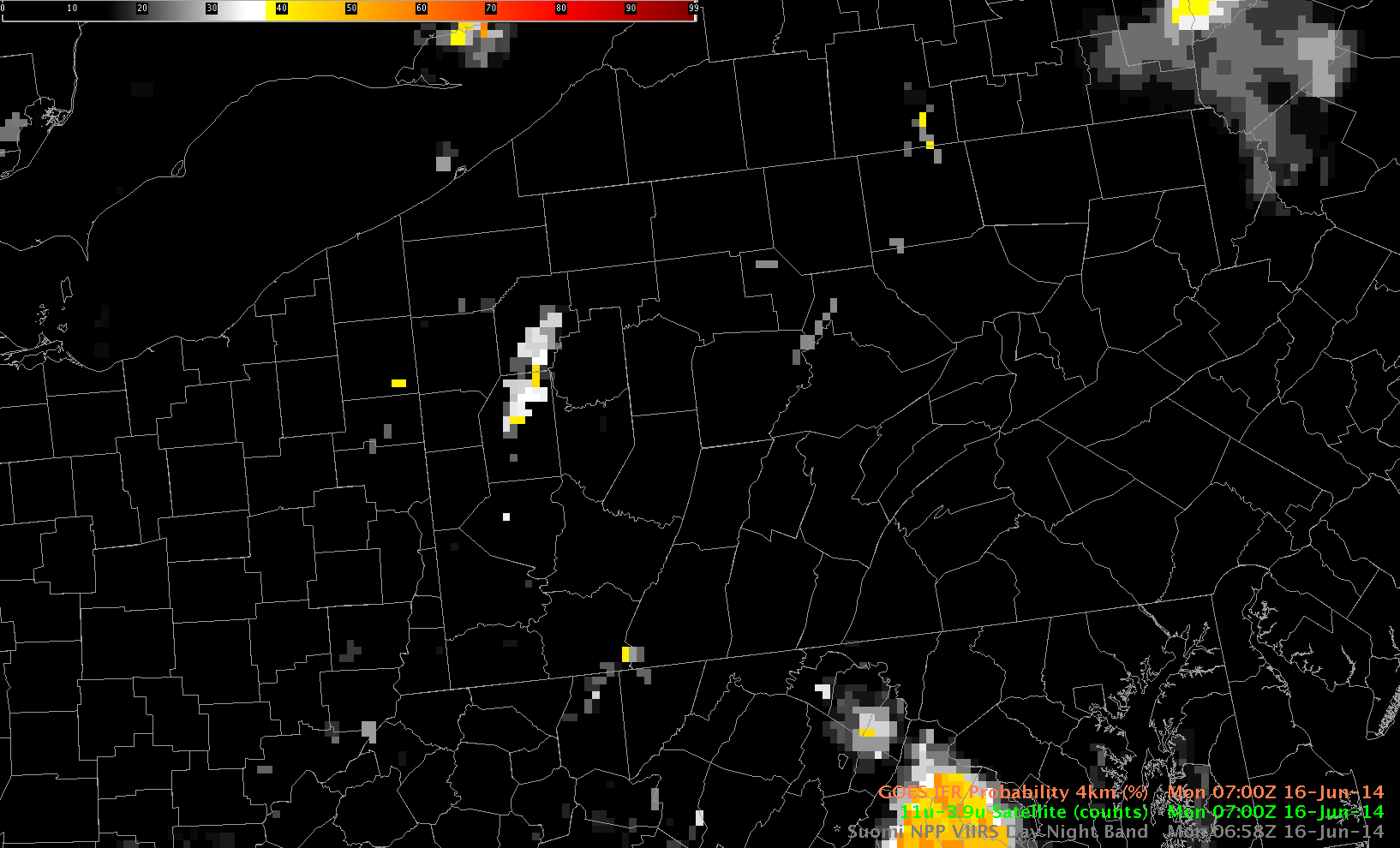
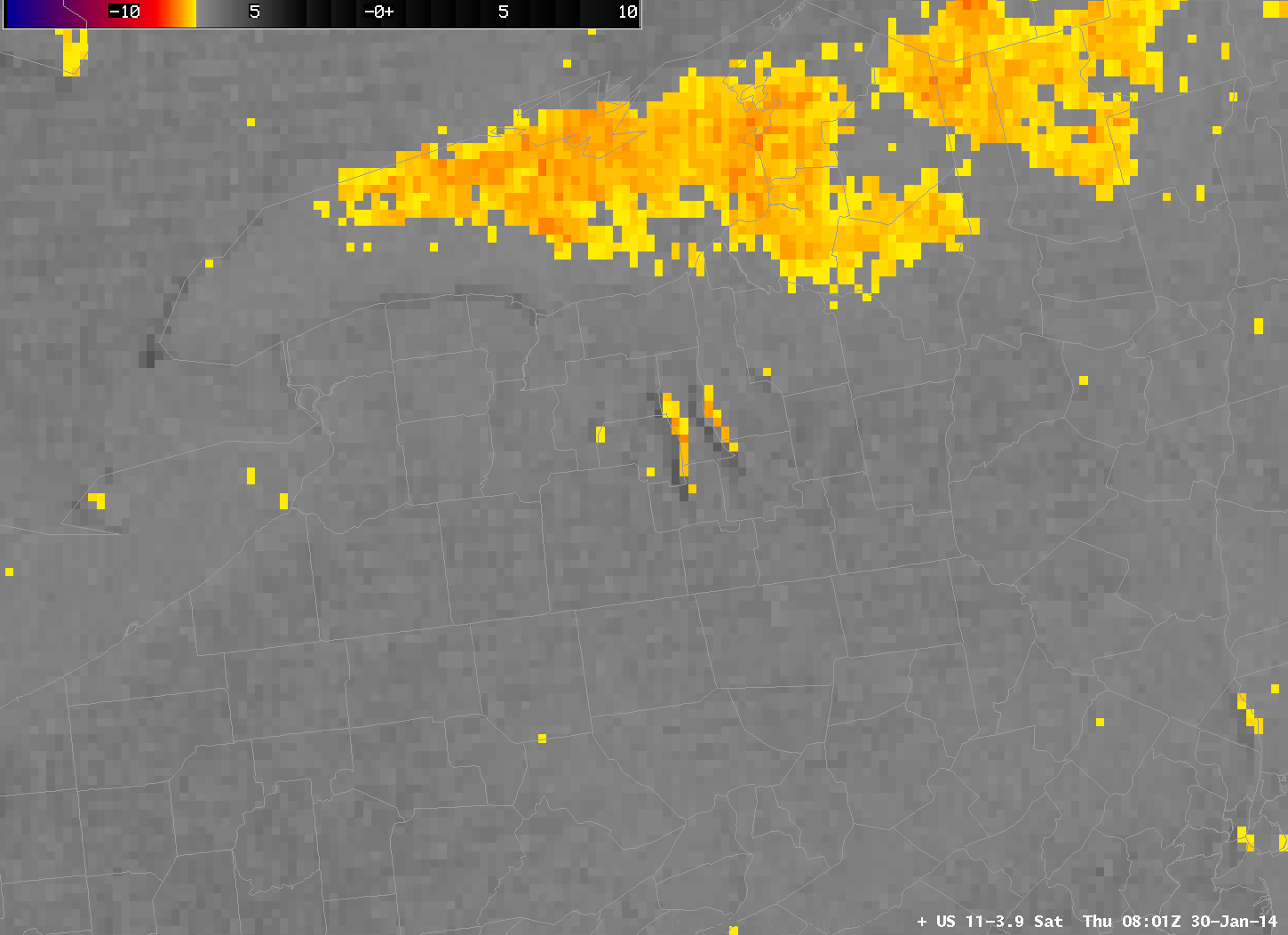
Suomi/NPP Day/Night Band and Brightness Temperature Difference (11.35 – 3.74) at 0658 UTC on 16 June 2014 (Click to enlarge)

Suomi/NPP Day/Night band “Visible Imagery at Night” from last night at 3 AM EDT over Pennsylvania and surrounding states shows cloud formation in the river valleys of Pennsylvania and New York. The brightness temperature difference also shows these cloud formations, but note over eastern New York how high cirrus prevents the detection of low clouds in river valleys using the brightness temperature difference field, but the cirrus is thin enough that the Day/Night band does show the low clouds. The brightness temperature difference field can show where clouds are present in regions where city lights in the day/night band might appear similar to clouds on a night when lunar illumination is strong (as was the case on 16 June 2014) — for example, along US Highway 220 from Lock Haven to Jersey Shore and Williamsport in southern Clinton and Lycoming Counties.

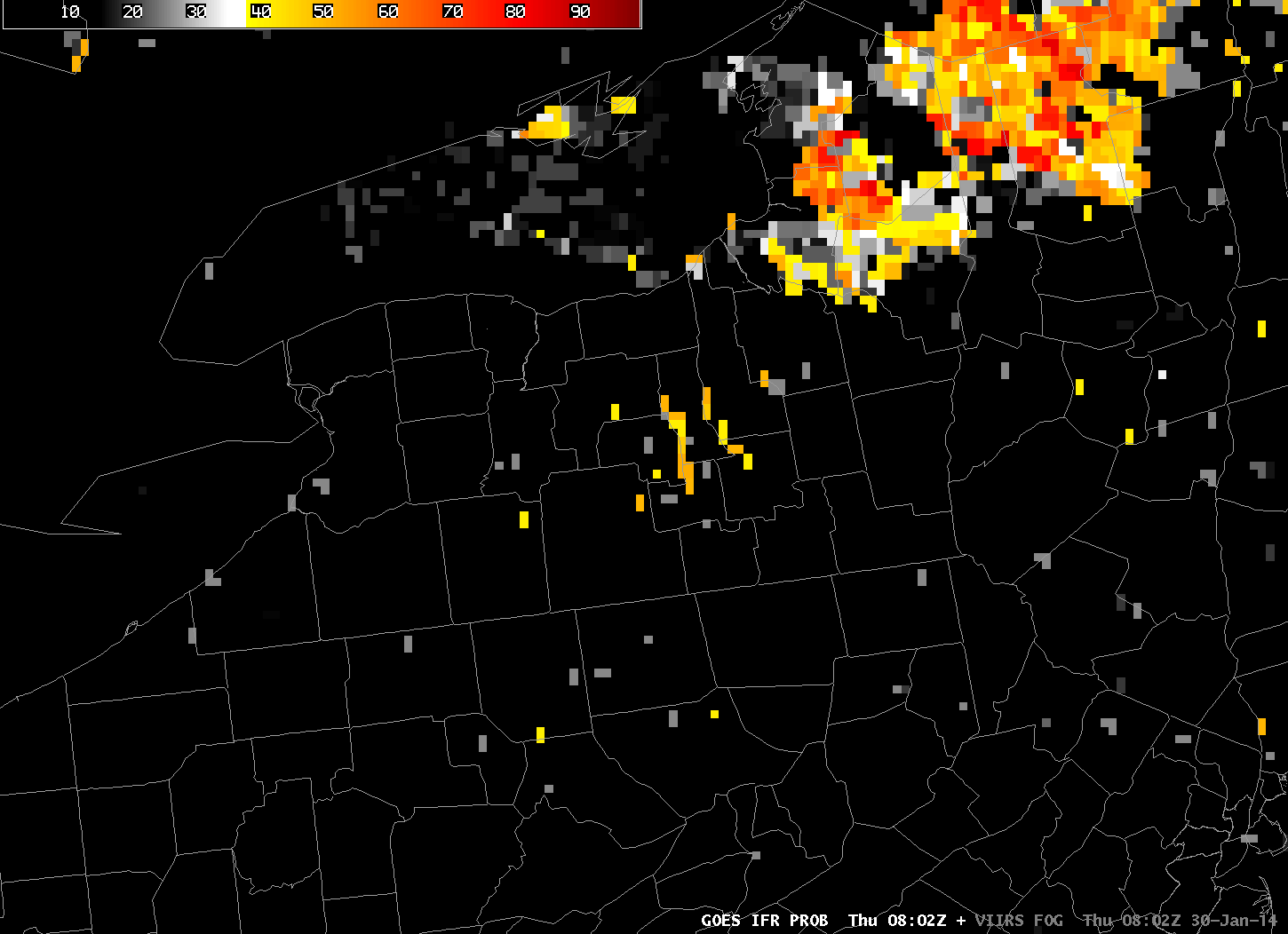
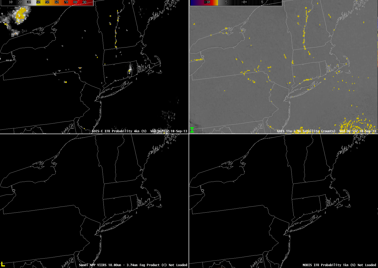
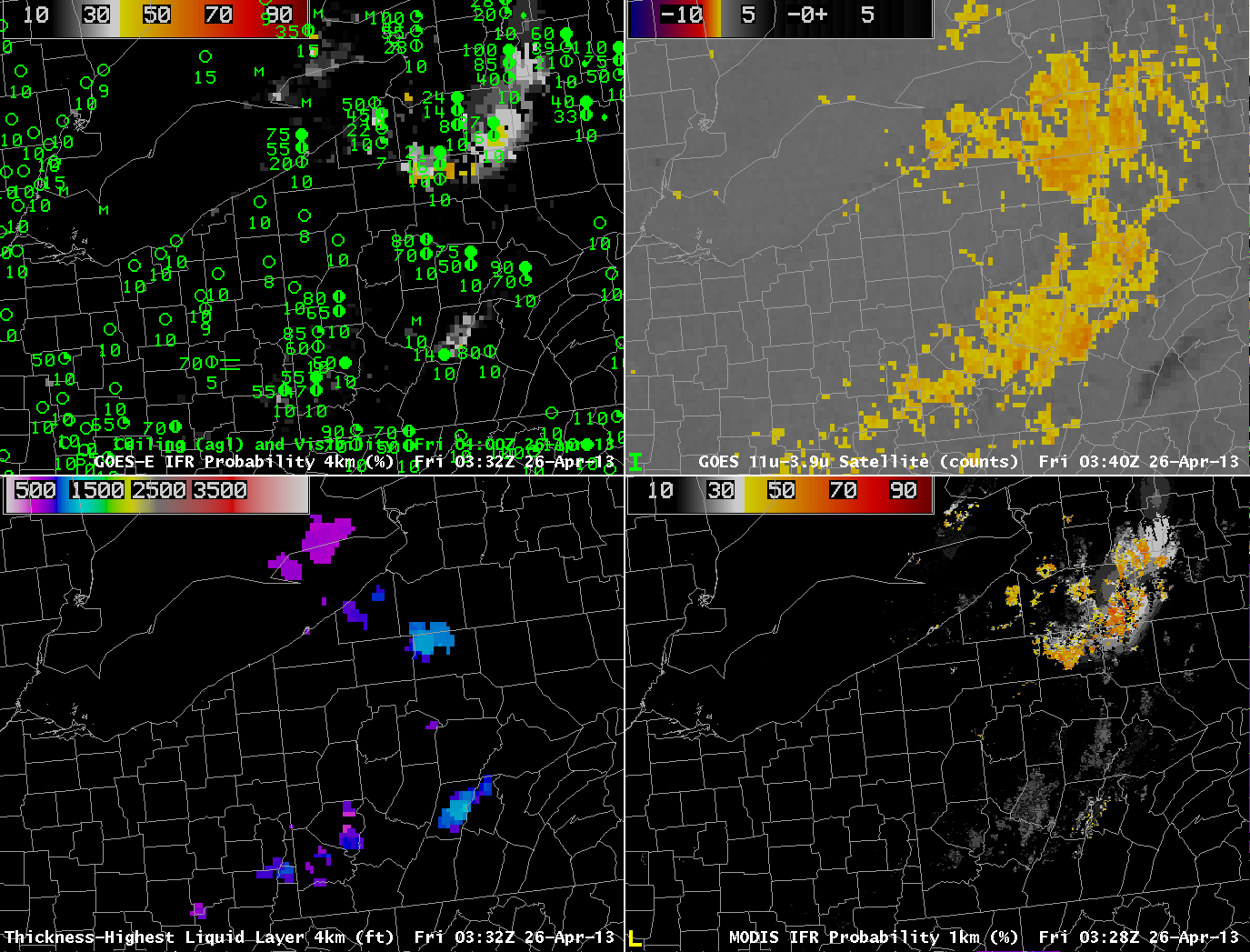
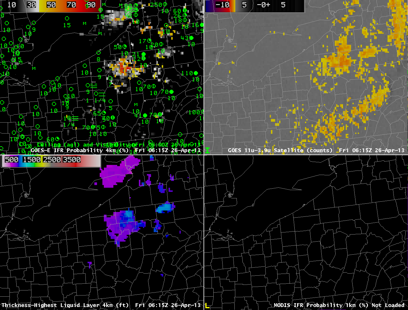
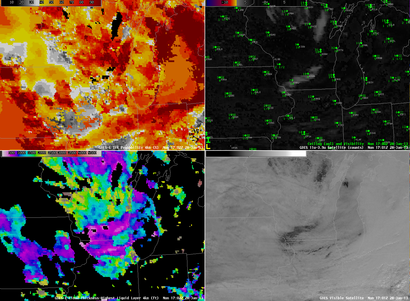
Of course, the Suomi/NPP satellite is seeing the top of the cloud, so it can be difficult to infer ceiling and visibility obstructions from these data. The GOES-based IFR Probability field from about the same time, below, shows hints of visibility restrictions, but the coarser resolution of GOES-13 (compared to Suomi/NPP) limits the ability of GOES to herald the development of fog. In addition, the 13-km resolution of the Rapid Refresh model data that are also used in the GOES-R IFR Probability fields is insufficient to resolve the small river valleys (such as Pine Creek that shows up very well in the S/NPP imagery in western Lycoming County). Portions of the Susquehanna River basins do show marginally enhanced probabilities, certainly something that would alert a forecaster to the possibilities of fog.

GOES-based IFR Probabilities, 0700 UTC on 16 June 2014 (Click to enlarge)

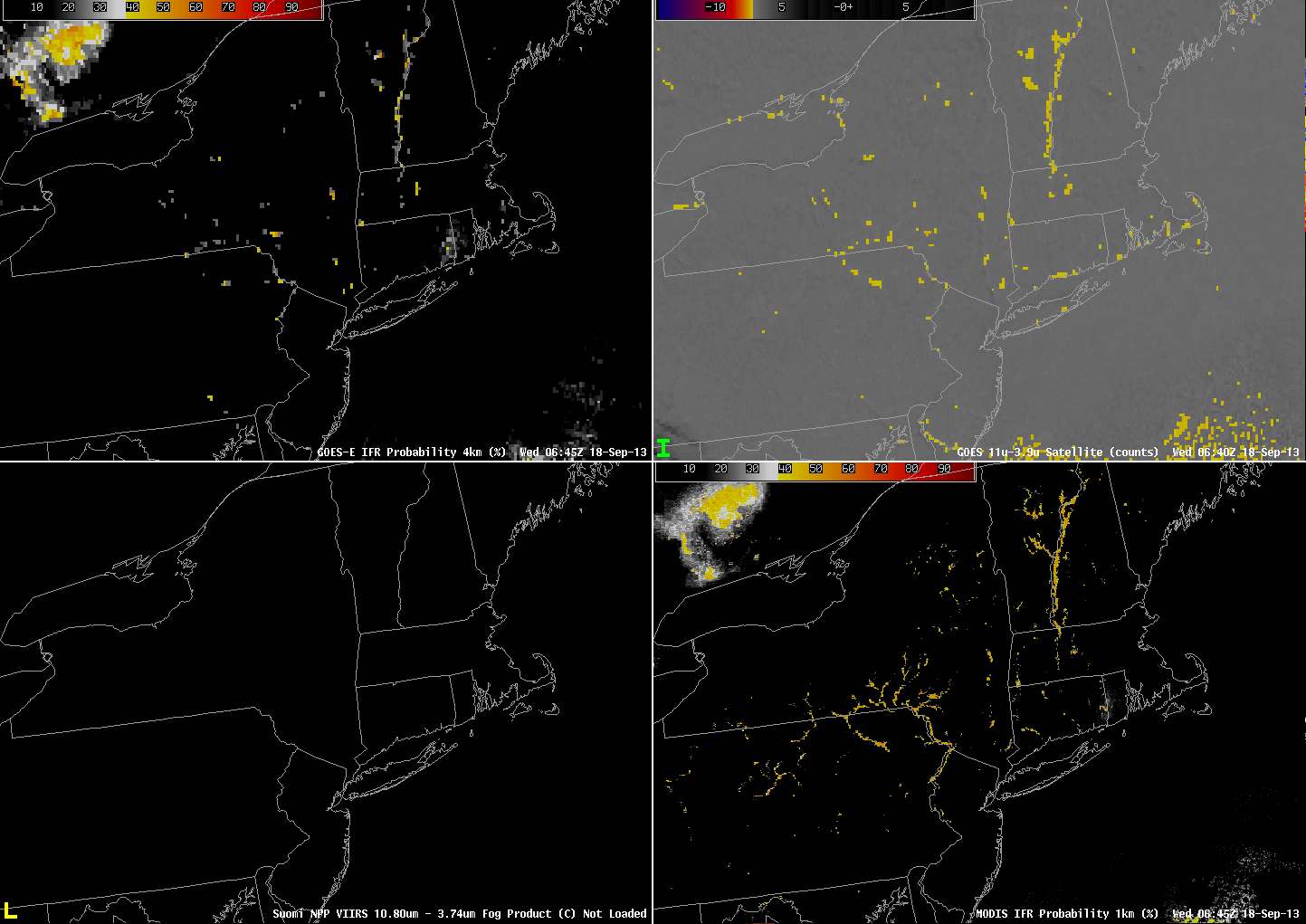
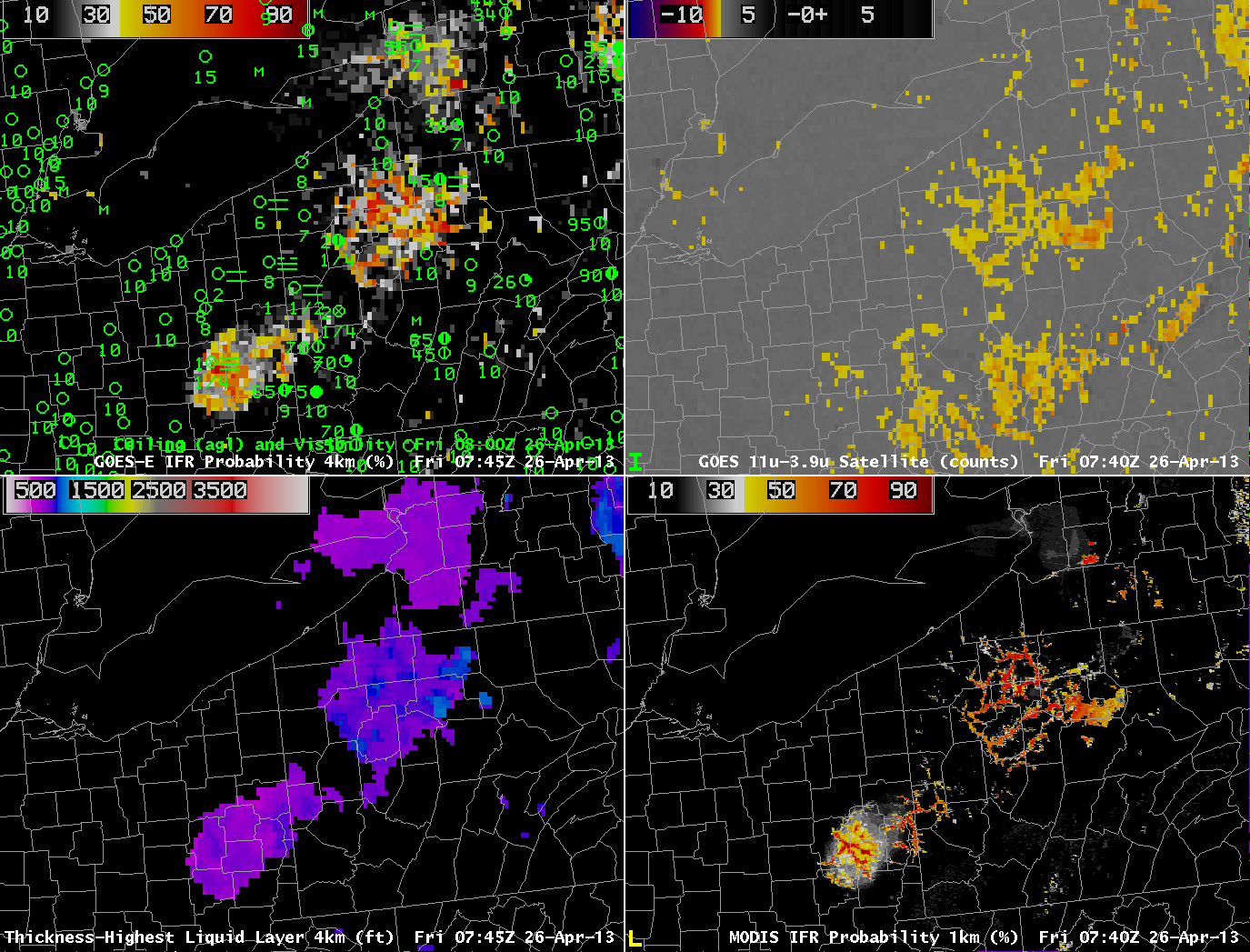
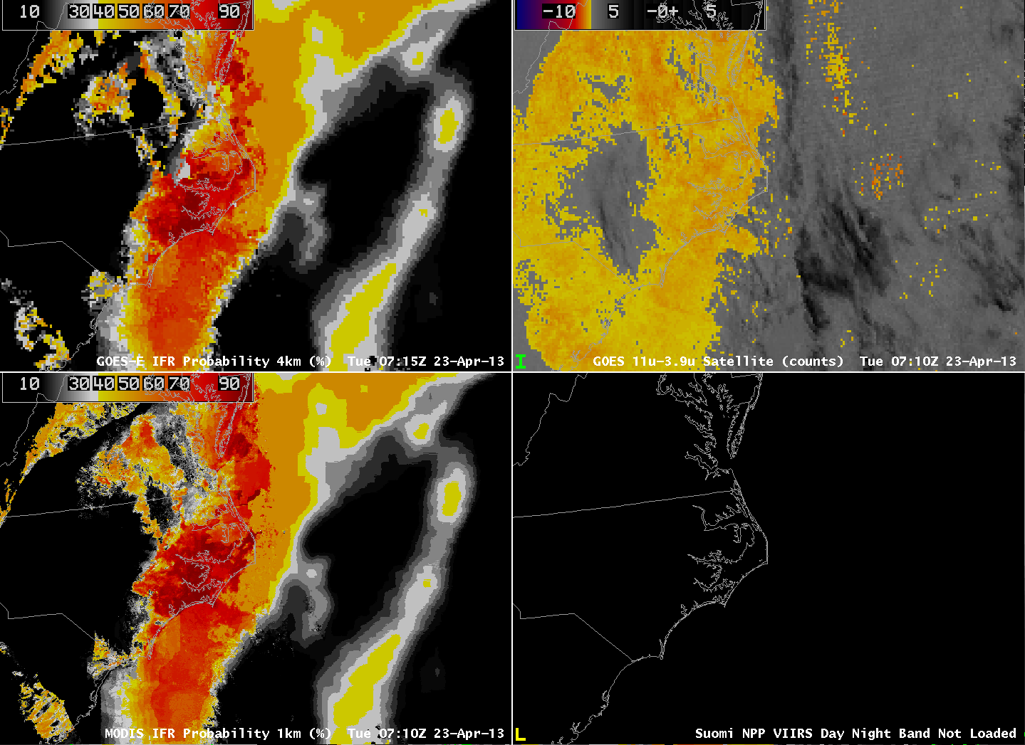
MODIS data can also be used to produce IFR Probabilities at infrequent intervals, but a timely overpass at 0744 UTC shows high probabilities in most of the river valleys of central Pennsylvania and upstate New York, with the highest probabilities near Elmira, NY.

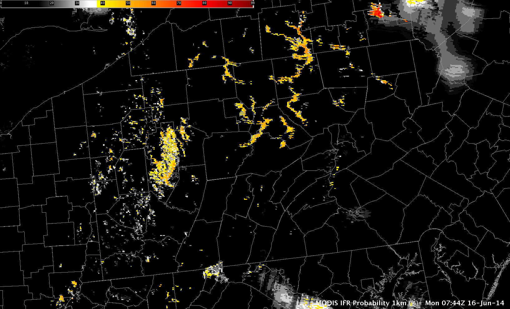
MODIS-based IFR Probabilities, 0744 UTC on 16 June 2014 (Click to enlarge)

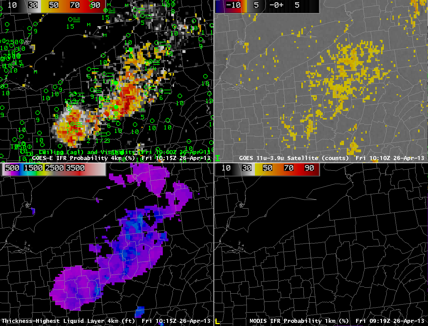
The GOES-R IFR Probabilities at 1000 UTC, below, show evidence that the fog/low stratus have become widespread enough in river valleys to be detected even by GOES. Elmira, NY, is reporting IFR conditions, and such conditions are also likely elsewhere in the valleys (although no observations are available to confirm that).

GOES-based IFR Probabilities, 1000 UTC on 16 June 2014 (Click to enlarge)

Use timely polar-orbiting satellite data — with high resolution — to confirm suspicions of developing fog in river valleys. Then monitor the situation with the good temporal resolution of GOES. During the GOES-R era, geostationary satellite spatial resolution will be increased and fog detection from GOES-R should occur with better lead time.

Radiation fog over coastal North Carolina

GOES-R IFR Probabilities with observations of ceilings/visibilities (Upper Left), GOES-East Brightness Temperature Difference (10.7µm – 3.9µm) (Upper Right), GOES-R Cloud Thickness (Lower Left), Suomi/NPP VIIRS Day/Night Band (0.70 µm, at night) or GOES-East Visible imagery (0.63 µm, during day), Times as indicated (Click to enlarge)

Clear skies allowed for radiation fog with IFR conditions to develop over eastern North Carolina overnight. GOES-R Cloud Thickness as observed at the last time before twilight conditions begin — in this case at 1000 UTC (6 AM EDT) — can be used as a predictor for fog dissipation time using this chart. At 1000 UTC, maximum cloud thickness was 1000 feet, which suggests a dissipation time around 1300-1330 UTC.

The visible animation, below, is in agreement with the prediction from the cloud thickness field.

GOES-East Visible Imagery (0.62 µm) Times as indicated (Click to enlarge)

A toggle of two images with Day/Night band imagery, below, shows the difficulty in using the Day/Night band to identify regions of fog/low clouds consistently. In the 0615 UTC image, the developing low clouds show up well (Of course, it’s hard to tell if the clouds are low stratus or mid-level stratus), but the picture at 0745 UTC is a lot less distinct.

GOES-R IFR Probability signal because of co-registration errors

GOES-R IFR Probabilities at 0802 UTC, 30 January 2014 (click image to enlarge)

Special Update, 17 November 2014.

GOES-R IFR Probabilities on the morning of 30 January suggested the likelihood of fog along some of the Finger Lakes of upstate New York. These high probabilities arise because the Brightness Temperature Difference (10.7 µm – 3.9 µm) Product, below, shows a signal there. Note, however, that the Brightness Temperature Difference has a shadow; this is the sign that the co-registration error that is present between the 10.7 µm and 3.9 µm channels is producing a fictitious signal of fog over the lake. Such errors have been discussed here and elsewhere in the past.

GOES-East Brightness Temperature Difference (10.7 µm – 3.9 µm) at 0801 UTC, 30 January 2014 (click image to enlarge)

Evidence that fog is not present is available in Suomi/NPP data taken at the same time as the GOES data, above. The toggle, below, of Day/Night Band imagery and of the brightness temperature difference (11.35 µm – 3.74 µm) from VIIRS shows scant evidence of fog/low stratus near the Finger Lakes. Because the moon is new, lunar illumination is at a minimum and surface features in the Day/Night band are not distinct, but the dark waters of the lakes are apparent.

Suomi/NPP VIIRS Day/Night band and Brightness Temperature Difference (11.35 µm – 3.74 µm) at 0802 UTC, 30 January 2014 (click image to enlarge)

MODIS data also suggests no fog/low stratus in the region. Both the brightness temperature difference field and the MODIS-based IFR Probabilities, below, support a forecast that does not mention fog around the Finger Lakes.

MODIS Brightness Temperature Difference (11 µm – 3.74 µm) and MODIS-based GOES-R IFR Probabilities at 0746 UTC, 30 January 2014 (click image to enlarge)

=====================================================================

Update, 17 November 2014

NOAA/NESDIS has tested a software fix to align better the longwave infrared (10.7 µm) and shortwave infrared (3.9 µm) channels. The toggle below is of the Brightness Temperature Difference Field with (After co-registration correction) and without (Prior to co-registration correction) the realignment.

GOES-13 Brightness Temperature Difference Fields at 0802 UTC, 30 January 2014, with and without the co-registration correction as indicated (Photo Credit: UW-Madison CIMSS; Click to enlarge)

The correction of the co-registration error translates into more realistic IFR Probabilities in/around the Finger Lakes. In this case, IFR Probabilities are reduced because the false strong signal from the satellite is not present because of more accurate co-registration.

GOES-R IFR Probability fields computed Prior to and After co-registration correction, data from 0802 UTC 30 January 2014. IFR Probability fields with the corrected co-registration data are more accurate. (Photo Credit: UW-Madison CIMSS; Click to enlarge)

Dense fog on the East Coast

GOES-East IFR Probabilities and surface plots of visibilities/ceilings at 0615 UTC 15 January (Upper Left), GOES-East Brightness Temperature Difference (10.7 µm – 3.9 µm), 0615 UTC 15 January (Upper Right), GOES-R Cloud Thickness, 0615 UTC 15 January (Lower Left), and Suomi/NPP Day/Night Band and Brightness Temperature Difference toggle (11.35 µm – 3.74 µm), 0605 UTC 15 January (Lower Right)(click image to enlarge)

The image above documents the GOES-R IFR Probability field during a fog event over the East Coast. Note how the IFR Probability field shows more horizontal uniformity than the traditional brightness temperature difference field over eastern Pennsylvania (where IFR conditions are reported). For example, both Selinsgrove along the Susquehanna and Reading in south-central Pennsylvania report IFR conditions in regions where the IFR Probability field has a strong return, but where the brightness temperature difference field’s diagnosis is less certain.

The Suomi/NPP field demonstrates the importance of higher resolution from polar orbiting satellites. Both the Day/Night Band and the brightness temperature difference fields suggest the presence of river valley fog over the West Branch of the Susquehanna and its many tributaries in central Pennsylvania. This continues at 0743 UTC, below, when Suomi/NPP’s subsequent overpass also viewed the Susquehanna valley. At both times, the river fog is too small-scale to be detected with GOES-13’s nominal 4-km pixel size.

GOES-East IFR Probabilities and surface plots of visibilities/ceilings at 0745 UTC 15 January (Upper Left), GOES-East Brightness Temperature Difference (10.7 µm – 3.9 µm), 0745 UTC 15 January (Upper Right), GOES-R Cloud Thickness, 0745 UTC 15 January (Lower Left), and Suomi/NPP Day/Night Band and Brightness Temperature Difference toggle (11.35 µm – 3.74 µm), 0743 UTC 15 January (Lower Right)(click image to enlarge)

The animation of the fields, below, done to demonstrate the importance of GOES-13’s temporal resolution, shows how the GOES-R IFR Probability field accurately captures the extent of the fog, even as the sun rises and causes the sign of the brightness temperature difference to flip. The traditional brightness temperature difference field has difficulty both in maintaining a signal through sunrise, and it diagnosing the region of fog/low stratus over northcentral Pennsylvania in and around the Poconos and in the Susquehanna River valley. The IFR Probability field has a minimum over/around Mt. Pocono, where IFR conditions are not observed until close to sunrise. IFR probabilities are small over Altoona, where the brightness temperature difference field shows a strong signal developing late at night (and where observations suggest an elevated stratus deck). In this region, although the satellite suggests fog might be present, model conditions do not agree, and IFR Probabilities are correctly minimized.

GOES-R Cloud thickness suggests that the thickest blanket of fog is over New Jersey. This diagnosis continues up through the twilight conditions of sunrise, at which point Cloud thicknesses are no longer diagnosed.

GOES-East IFR Probabilities and surface plots of visibilities/ceilings (Upper Left), GOES-East Brightness Temperature Difference (10.7 µm – 3.9 µm) (Upper Right), GOES-R Cloud Thickness (Lower Left), and GOES-East Water Vapor (6.7 µm), all times as indicated (Lower Right)(click image to enlarge)

GOES Resolution might miss valley fog (Plus: What does Stray Light look like?)

GOES-R IFR Probability (Upper Left), GOES-East Brightness Temperature Difference (Upper Right), Suomi/NPP Brightness Temperature Difference (Lower Left), MODIS-based IFR Probability (Lower Right), all imagery at 0615 UTC on 18 September 2013 (click image to enlarge)

Nominal GOES resolution for the Brightness Temperature Difference product that is used in the GOES-R IFR Probability is 4 km at the sub-satellite point, and it worsens as you move into mid-latitudes. Rapid Refresh Model resolution is even coarser than the satellite. When fog is forming in narrow valleys, then, there can be a significant lag in the time from when it starts to form to when the satellite data, and the satellite/model fused product, detects it. In the 0615 UTC image above, for example, only a few pixels of strong GOES-detected Brightness Temperature Difference, and enhanced IFR Probabilities, exist. In the 0630 UTC image, below, there has been little change in the GOES-based imagery. However, the Suomi/NPP data at the time, at 1-km resolution, suggests fog is forming in many of the river valleys of Pennsylvania, but it is still sub-gridscale as far as GOES can detect.

GOES-R IFR Probability (Upper Left), GOES-East Brightness Temperature Difference (Upper Right), Toggle between Suomi/NPP Day/Night band imagery and Suomi/NPP Brightness Temperature Difference (Lower Left), MODIS-based IFR Probability (Lower Right), all imagery at ~0630 UTC on 18 September 2013 (click image to enlarge)

GOES-R IFR Probability (Upper Left), GOES-East Brightness Temperature Difference (Upper Right), Suomi/NPP Brightness Temperature Difference (Lower Left), MODIS-based IFR Probability (Lower Right), all imagery at 0645 UTC on 18 September 2013 (click image to enlarge)

Fifteen minutes later, the MODIS-based IFR probabilities (above) suggest a strong possibility of IFR conditions in many of the river valleys of Pennsylvania. However, Suomi/NPP and MODIS data come from polar orbiters so that high resolution information is infrequent. When GOES-R is launched, ABI will have nominal 2-km resolution in the infrared, which resolution is intermediate between GOES and MODIS.

The higher-resolution polar orbiters’ occasional views can give a forecaster an important heads’ up for fog formation. By 0815 UTC the GOES-based information is showing higher IFR probabilities in the river valleys of Pennsylvania, but a Suomi/NPP overpass shows that it is still underestimating the areal extent of the fog.

GOES-R IFR Probability (Upper Left), GOES-East Brightness Temperature Difference (Upper Right), Toggle between Suomi/NPP Day/Night band imagery and Suomi/NPP Brightness Temperature Difference (Lower Left), MODIS-based IFR Probability (Lower Right), all imagery at ~0815 UTC on 18 September 2013 (click image to enlarge)

Note that this is a time of year when stray light does occasionally enter the GOES signal, causing contamination. This occurred — and was very obvious — around 0400 UTC on 18 September. As is typical, it was present for only one scan. See below.

GOES-R IFR Probability (Upper Left), GOES-East Brightness Temperature Difference (Upper Right), GOES-R Cloud Thickness (Lower Left), MODIS-based IFR Probability (Lower Right), all imagery at ~0815 UTC on 18 September 2013 (click image to enlarge)

Radiation Fog over the Allegheny Mountains of Pennsylvania

Leave a reply

GOES-R IFR Probabilities computed using GOES-East data, hourly from 0400 UTC through 1000 UTC (excluding 0500 UTC), 26 April 2013

GOES-R IFR Probabilities show a region over the Allegheny Mountains of northwest Pennsylvania slowly acquiring higher and higher probabilities, as ceilings and visibilities drop. How did this product perform relative to traditional fog detection imagery (the brightness temperature difference product) and relative to data from Polar Orbiting satellites? (The 0500 UTC imagery is excluded from the animation above because Stray Light Contamination in the 3.9 channel was apparent in the IFR probability fields).

GOES-R IFR Probability computed from GOES-East, 0332 UTC (Upper Left), GOES-East Brightness temperature Difference field (10.7µm – 3.9µm) at 0340 UTC (Upper Right), GOES-R Cloud Thickness (Lower left), GOES-R IFR Probability computed from MODIS data, 0328 UTC (Lower Left).

The ‘traditional’ method of fog detection that exploits emissivity difference of water clouds at 10.7µm and 3.9 µm, upper right in the figure above, at about 0330 UTC, just as the radiation fog was starting to develop, shows clouds detected over north-central Pennsylvania, but also from Centre County southwestward to the Laurel Highlands and to West Virginia. GOES-based and MODIS-based IFR Probability fields have very low probabilities with these primarily mid-level clouds.

As above, but at 0615 UTC 26 April 2013

By 0615 UTC, IFR probabilities continue to increase over north-central Pennsylvania, and they remain low over southern and central Pennsylvania where mid-level clouds are reported (4100-foot ceilings at Johnstown, for example).

As above, but at 0740 UTC 26 April 2013

Another MODIS overpass at 0740 UTC better resolves the character of the developing fog and low stratus over north-central Pennsylvania. Very high IFR probabilities in the MODIS-based fields outline the river valleys of the Allegheny Plateau in north-Central Pennsylvania. GOES-based IFR Probabilities are high, but GOES lacks the resolution to view clearly the individual river valleys.

As above, but with Suomi/NPP brightness temperature difference (10.8 µm- 3.74µm) and Day-Night Visible imagery in the bottom right (0652 UTC), with the GOES-R IFR Probabilities (Upper Left), GOES-E Brightness Temperature Difference field (Upper Right), and GOES-R Cloud Thickness toggling between 0645 and 0702 UTC.

Suomi/NPP can also give information at high resolution about the evolving fog field. The tendrils of fog developing in the river valleys are evident in the visible imagery created using reflected lunar illumination (A mostly full moon was present the morning of 26 April) and those water-based clouds are also highlighted in the Suomi/NPP Brightness Temperature Difference Field. The clouds over the Laurel Highlands are higher clouds — they are casting shadows visible in the Day/Night band.

As in the figure above, but for 1015 UTC 26 April 2013

The final GOES-R Cloud Thickness field before twilight conditions, above, shows maximum thicknesses of 900 feet over Warren County, Pennsylvania, and around 850 feet over southern Clarion County. According to this link, such a radiation fog will burn off in less than 3 hours after sunrise. The animation below of visible imagery at 1315 and 1402 UTC shows the fog, initially widespread in river valleys at 1315 UTC mostly gone by 1402 UTC.

GOES-13 Visible Imagery, 1315 and 1402 UTC, 26 April 2013. Warren and Clarion Counties are highlighted.

Fog over coastal North Carolina

Leave a reply

GOES-R IFR Probabilities computed from GOES-East data, hourly from 0100 through 1200 UTC, 23 April 2013

A coastal storm along the east coast was responsible for low-level moisture over eastern North Carolina that resulted in IFR conditions. Multiple cloud layers in the beginning of the animation above mean that IFR probabilities were computed using model data. By 0315 UTC, however, upper level clouds had moved off the coast, leaving behind clouds at low layers that meant cloud data (brightness temperature difference) could influence the IFR probability fields; consequently, the probability increased. High clouds remained offshore, however, and the character of the IFR probability field shows the characteristic pixelated appearance over land — where satellite data are used in the computation of IFR probabilities — and the characteristic smoothed appearance over water where only model data are used to produce IFR probabilities. Note how the highest IFR probabilities over eastern North Carolina do overlap the stations reporting IFR and near-IFR conditions.

GOES-R IFR Probabilities (Upper Left) computed using GOES-East, GOES-East Brightness Temperature Difference (10.7 µm- 3.9µm) (Upper Right), GOES-R IFR Probabilities computed using MODIS data (Lower Left). All for times around 0715 UTC 23 April

The image above compares GOES-R IFR probabilities computed with MODIS and with GOES-East. They do show very similar overall structures, with highest probabilities over land where the Brightness Temperature Difference field can contribute to the probability, and lower, smoother probability fields over water where only model data are used. Note that both GOES-R IFR fields correctly ignore the low cloud signal over eastern South Carolina and central North Carolina.

GOES-R IFR Probabilities (Upper Left) computed using GOES-East, GOES-East Brightness Temperature Difference (10.7µm – 3.9µm) (Upper Right), Suomi/NPP Day/Night band from VIIRS (Lower Right). Toggle for times 0615 and 0745 UTC 23 April

The GOES-based IFR probability field can also be compared to the Day/Night band sensed by VIIRS on board Suomi/NPP. The 0609 UTC Day/Night band shows the effects of a near-full moon on the product. The extensive cloud shield east of the Appalachians is visible, even though the image is at night, because of strong lunar illumination. As with the traditional brightness temperature difference field, however, the cloud information from the Day/Night band gives little information about the cloud bases; for that, the IFR probability field is needed, and low cloud bases are correctly restricted to extreme eastern North Carolina. The Day/Night band at 0747 UTC is from a time after the moon has set; only city lights and airglow are illuminating the clouds over Virginia and the Carolinas. Cloud edges are still easily discerned.

Fog-related Crash on I-77 in southern Virginia

Leave a reply

GOES-R IFR Probabilities computed from GOES-East (Upper Left), MODIS Visible imagery and surface plots of ceilings/visibility (Upper Right), GOES-R IFR Probabilities computed from MODIS (Lower Left), MODIS 10.7 micron data (Lower Right), images at ~1630 and ~1815 UTC.

Seventeen separate crashes involving nearly 100 vehicles near milepost 5 on Interstate 77 in Carroll County in southern Virginia claimed three lives on Sunday March 31st. The crashes occurred in fog and started around 1 PM (1700 UTC). How did the Fog/Low Stratus product do in alerting forecasters to the presence of the fog? This case demonstrates the challenges inherent in Fog Detection. GOES-R IFR Probabilities show a distinct reduction in probabilities over the crash site in the times bracketing the crash time, above. An animation of GOES-based IFR probabilities, below, shows relatively high probabilities until just before the crash time, after which time probabilities dropped. Photographs from after the crash, during the clean-up, show that fog persisted into the afternoon hours.

GOES-R IFR Probabilities computed from GOES-East and Rapid Refresh Data, 1602-1815 UTC on 31 March 2013

Note that widespread fog is typically not associated with crashes. Rather, patchy fog that can be driven into from regions with greater visibility is a greater hazard. Such patchy fog is most likely to be sub-pixel scale.

IFR Probabilities during a Winter Storm

Leave a reply

GOES-R IFR Probabilities computed from GOES-East and Rapid Refresh model output, from 0100 through 1400 UTC on March 25 2013

A late winter storm moving through the mid-Altantic states was responsible for an episode of reduced visibilities. The loop above shows two areas of reduced visibilities initially — one over the Piedmont of Georgia, the Carolinas and Virginia, and one over the Ohio River Valley. Visibilities decrease as the higher IFR probabilities move in, and, conversely, increase as the higher probabilities move out. IFR Probabilities over southern Ohio, for example, have a character that suggests the probabilities have been computed chiefly with model data. Probabilities are somewhat reduced, and the fields are not pixelated (as they are over the Carolina Piedmont, for example).

GOES-R IFR Probabilities computed from GOES-East, Brightness Temperature Difference fields from GOES-East (10.7 µm – 3.9 µm) and from Suomi/NPP (10.8 µm- 3.74 µm) around 0700 UTC on 25 March 2013

The animation of the ~0700 UTC IFR Probability and brightness temperature difference field from both GOES-East and from the polar-orbiting Suomi/NPP, above, shows another strength of the IFR Probability product: It screens out regions where high stratus give a signal. The top of a stratus deck and the top of a fog deck may have a very similar brightness temperature difference signal. By fusing the satellite data with a product that includes surface information (such as output from the Rapid Refresh Model), regions with elevated stratus, which clouds do not significantly impact aviation operations, can be removed from the signal. Only regions with actual surface observation restrictions are highlighted in the IFR probability signal above.

Advection Fog in the Midwest

Leave a reply

GOES-R IFR Probabilities from GOES-East, hourly from 00:15 through 13:15 on 28 January 2013, with surface visibilities and ceilings.

Warm and moist air streaming north from the southern Plains has encountered the cold (and in some places) snow-covered ground. This is a time-honored recipe for advection fog, and the GOES-R IFR Probabilities fields, above, neatly capture the horizontal extent of the visibility restrictions overnight. The highest IFR Probabilities occur in regions where both Satellite Predictors and Model-based predictors are high. Note, for example, the somewhat lower probabilities that develop over Nebraska at the end of the animation. This is a region where higher clouds are moving in.

GOES-R IFR Probabilities (Upper Left), GOES-East Brightness Temperature Difference (10.7 µm – 3.9 µm) (Upper Right), GOES-R Cloud Thickness (Lower Left), GOES-East 10.7 µm Brightness Temperature (Lower Right)

Note how the Cloud Thickness product is not computed where the higher clouds are moving in. The product is computed only where single layer clouds are present in non-twilight conditions. Twilight conditions are present in the eastern half of the final image, at 1315 UTC. When radiation fog is present (rather than advection fog in this case), the last cloud thickness before twilight conditions can be used to estimate dissipation time using this chart.

GOES-R IFR Probabilities (Upper Left), GOES-East Brightness Temperature Difference (10.7 µm – 3.9 µm) (Upper Right), GOES-R Cloud Thickness (Lower Left), GOES-East Visible Imagery (0.62 µm) (Lower Right)

Holes in the advection fog developed around 1700 UTC.

GOES-R Fog Product Examples

Fog detection fusing GOES, Terra/Aqua or Suomi/NPP Satellite data with Model output

Category Archives: Mid-Atlantic

Fog in the Valleys of Pennsylvania and New York

Radiation fog over coastal North Carolina

GOES-R IFR Probability signal because of co-registration errors

Dense fog on the East Coast

GOES Resolution might miss valley fog (Plus: What does Stray Light look like?)

Radiation Fog over the Allegheny Mountains of Pennsylvania

Fog over coastal North Carolina

Fog-related Crash on I-77 in southern Virginia

IFR Probabilities during a Winter Storm

Advection Fog in the Midwest