 |
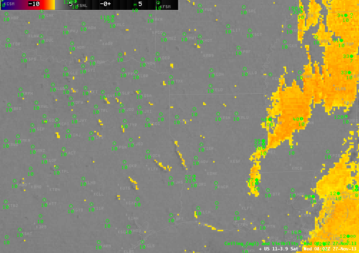
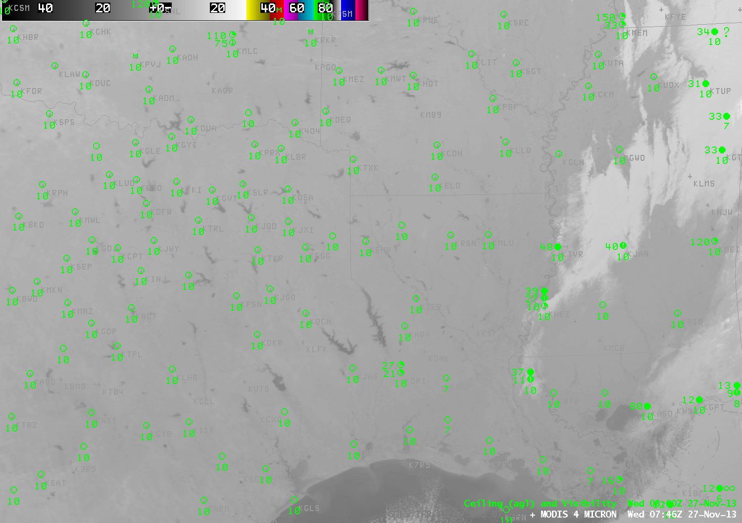
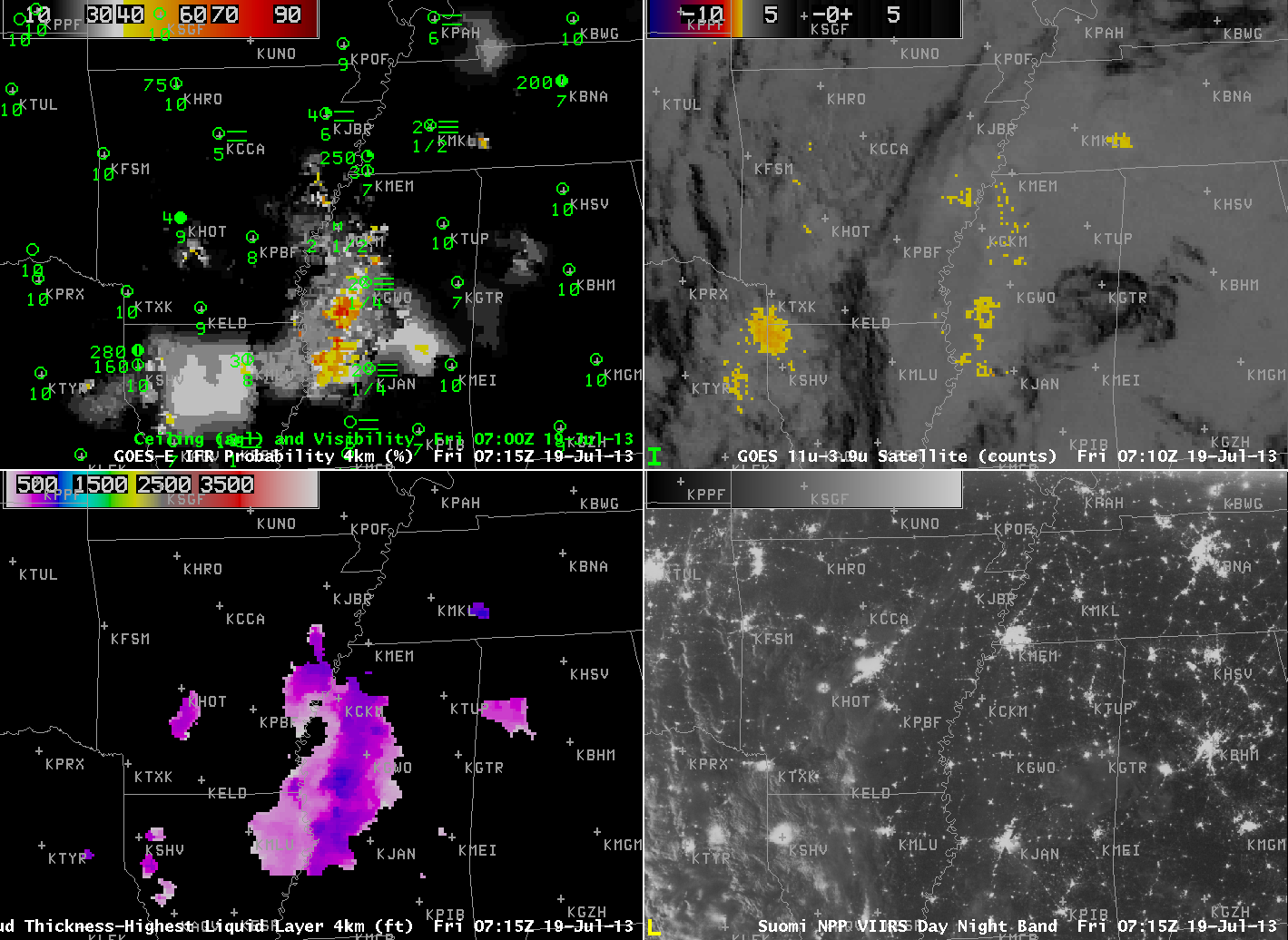
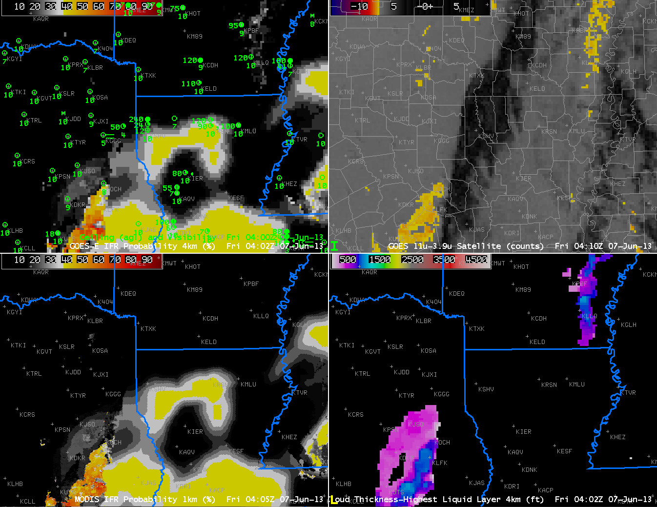
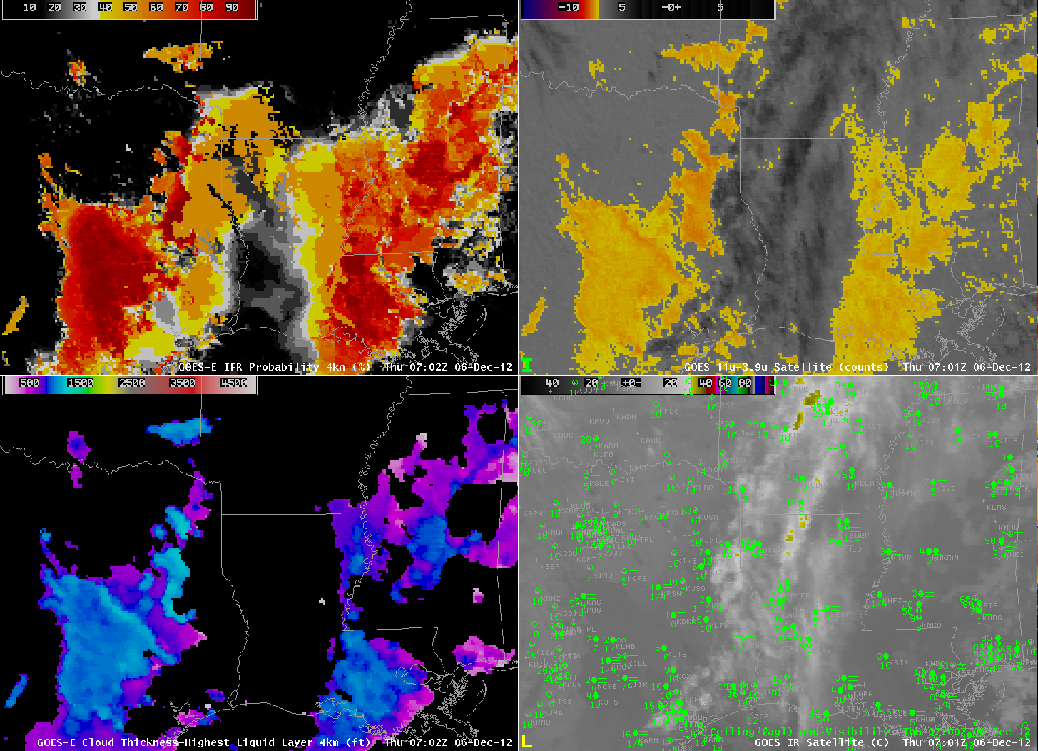
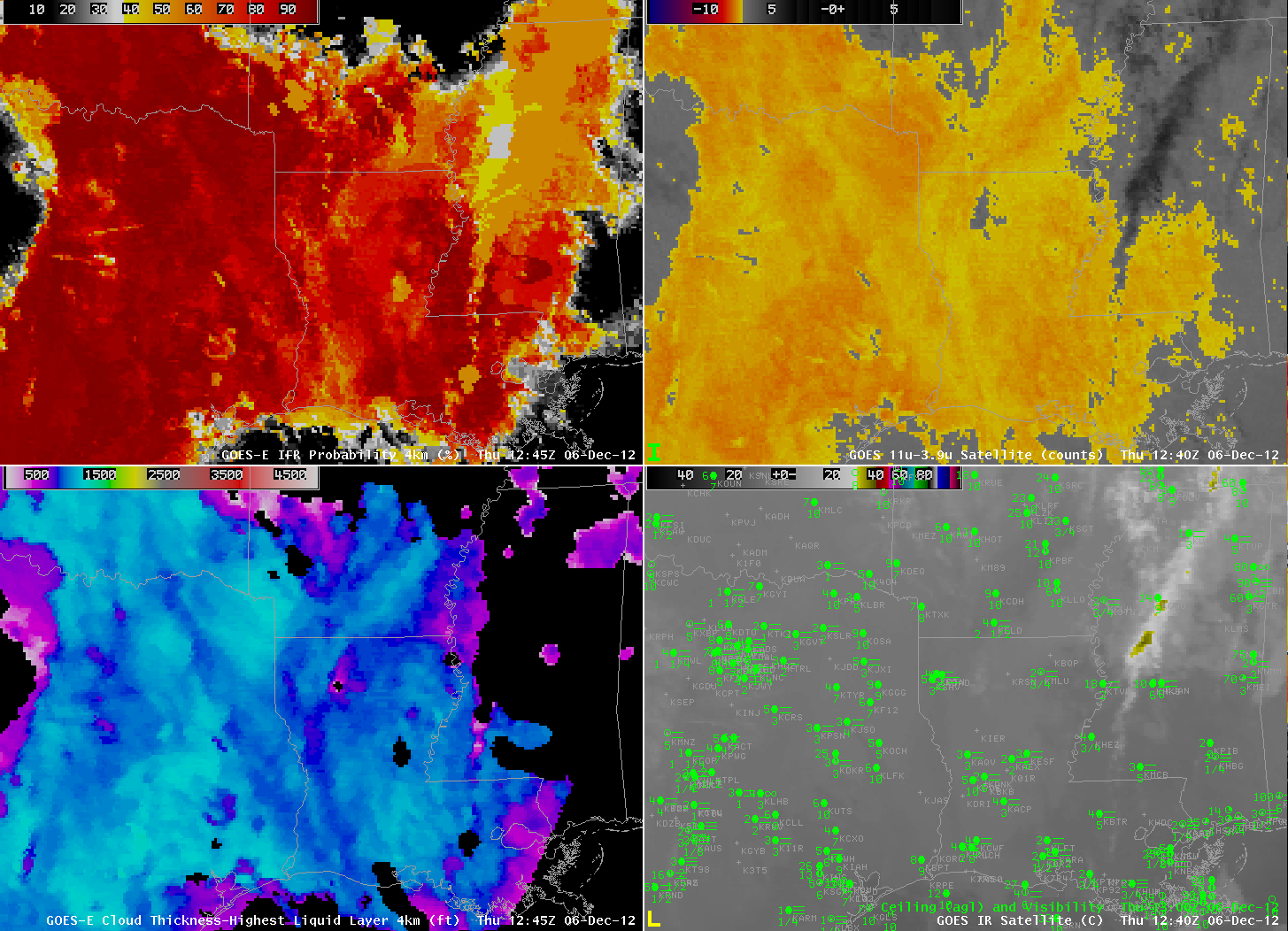
| GOES-R IFR Probabilities computed from GOES-East (Upper Left), GOES-East Brightness Temperature Difference (10.7 µm – 3.9 µm) (Upper Right), GOES-R Cloud Thickness (Lower Left), GOES-East 10.7 µm Imagery (Lower Right) at 0700 UTC on 6 December 2012. |
Upper-level clouds, such as those apparent in both the 10.7 µm imagery and the brightness temperature difference imagery, above, lower right and upper right, respectively, have an impact on the GOES-R IFR Probability and GOES-R Cloud Thickness products. The most obvious impact is in the Cloud Thickness product (lower left), which product is not computed in regions where high clouds are present. The GOES-R IFR Probabilities are computed underneath high clouds, using mostly Rapid Refresh model data to determine the probability of fog and low stratus. However, because cloud predictors are not used, IFR probabilities are somewhat lower. In addition, the character of the field is flatter, reflecting the smoother fields that are present in the model. This is especially obvious over northeast Louisiana and extreme east Texas in the IFR Probability image above. Thus, the heritage product, the brightness temperature difference, gives no information from southwest Louisiana northward into southern Arkansas, but the fused GOES-R IFR Probabilities do suggest enhanced possibilities of IFR conditions in regions where reduced visibilities are reported: central and northeast Louisiana and east Texas. IFR Probabilities are much lower over southwest Louisiana where IFR conditions are not reported.
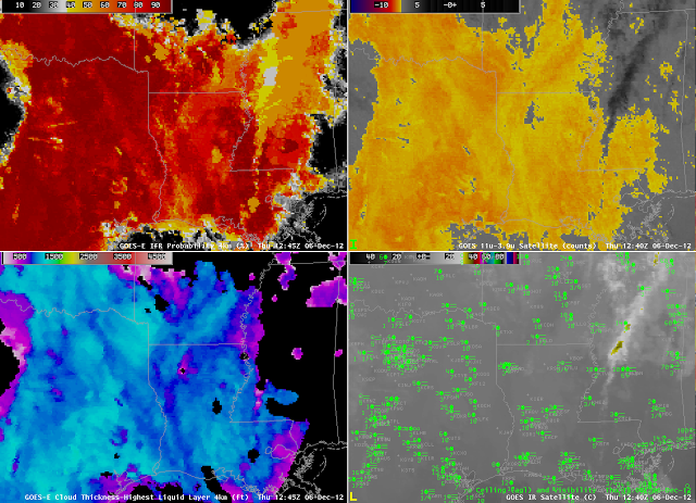 |
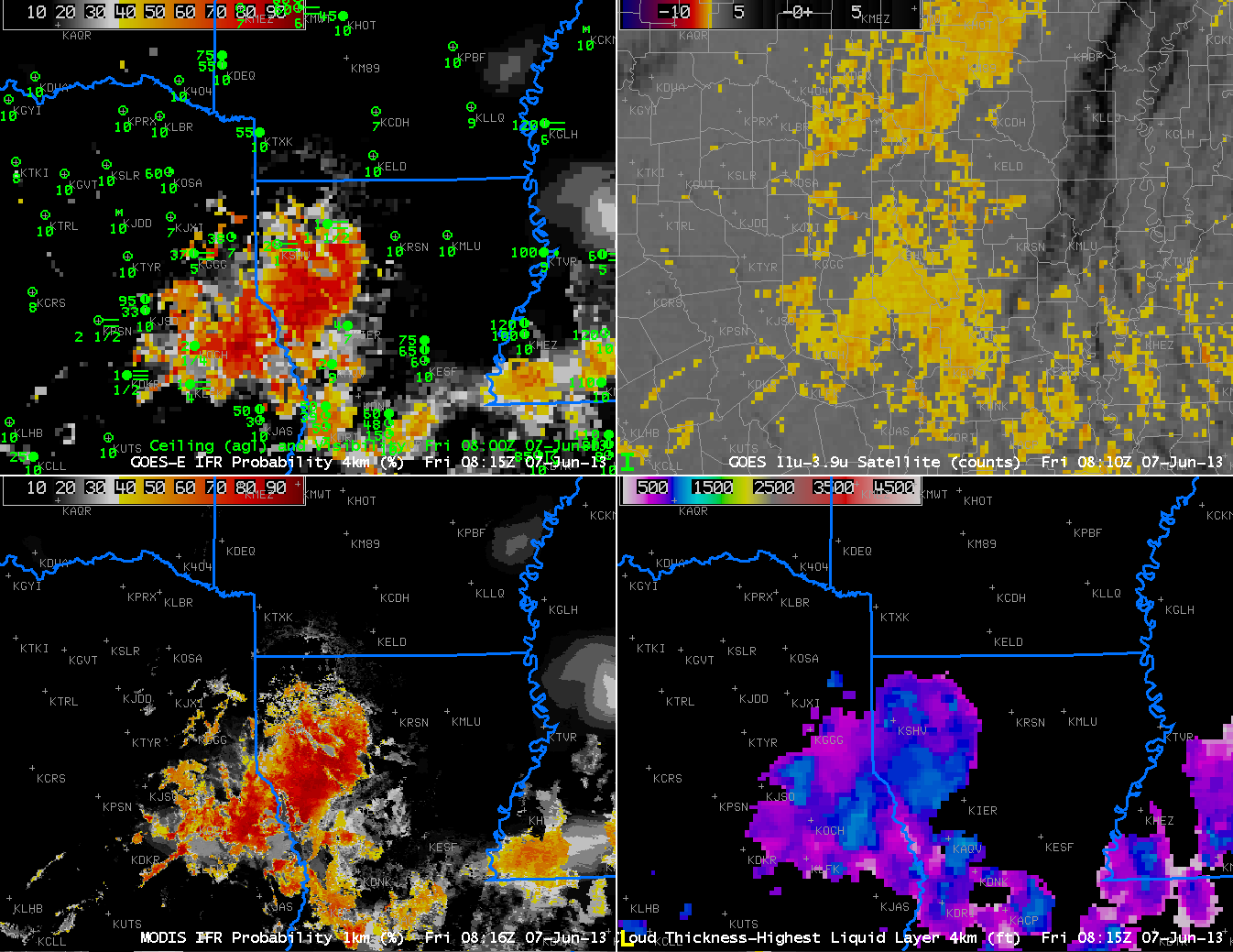
| As above, but for 1245 UTC on 6 December 2012. |
By 1245 UTC, the high clouds have lifted northeast and dissipated somewhat, so the heritage brightness temperature difference product gives information over the entire lower Mississippi River valley and over east Texas, where IFR conditions were widespread underneath very high GOES-R IFR Probabilities. The GOES-R Cloud Thickness product indicates cloud thicknesses up to near 1200 feet, suggesting a burn-off time for radiation fog of around 5 hours.
 |
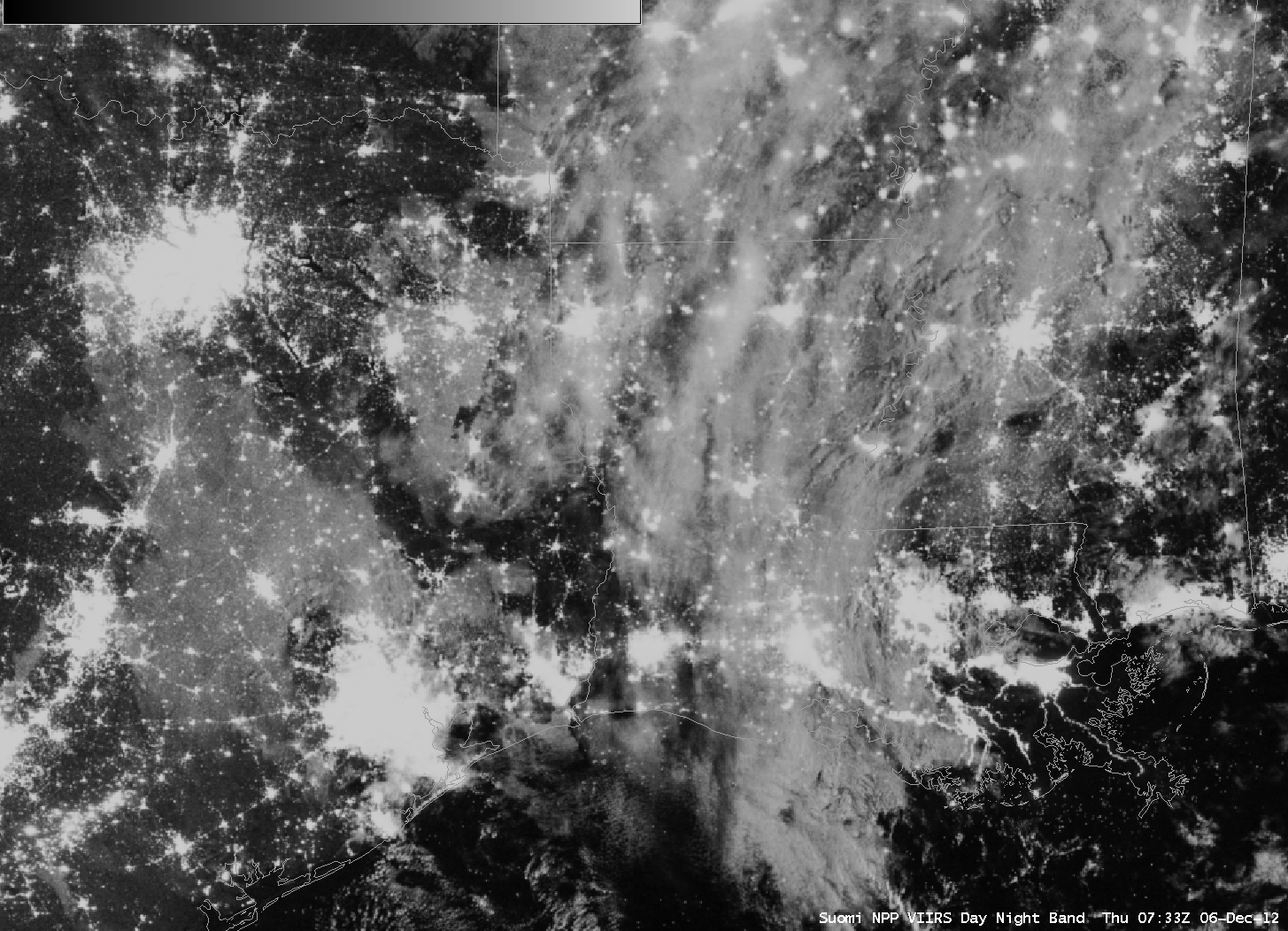
| Day/Night Band (from Suomi/NPP) imagery over Louisiana and East Texas, 0733 UTC on 6 December 2012. |
|
The Day/Night band image derived from data from Suomi/NPP from 0733 UTC on 6 December, above, shows the higher and lower clouds over Texas and Louisiana. The clouds between Houston and Dallas/Ft. Worth are low clouds, but the high clouds over Louisiana inhibit the detection of low clouds. In addition, although the Day/Night band can give a good outline of where the clouds are, it does not show where the visibility restrictions consistent with IFR conditions are.
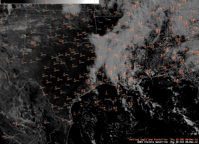 |
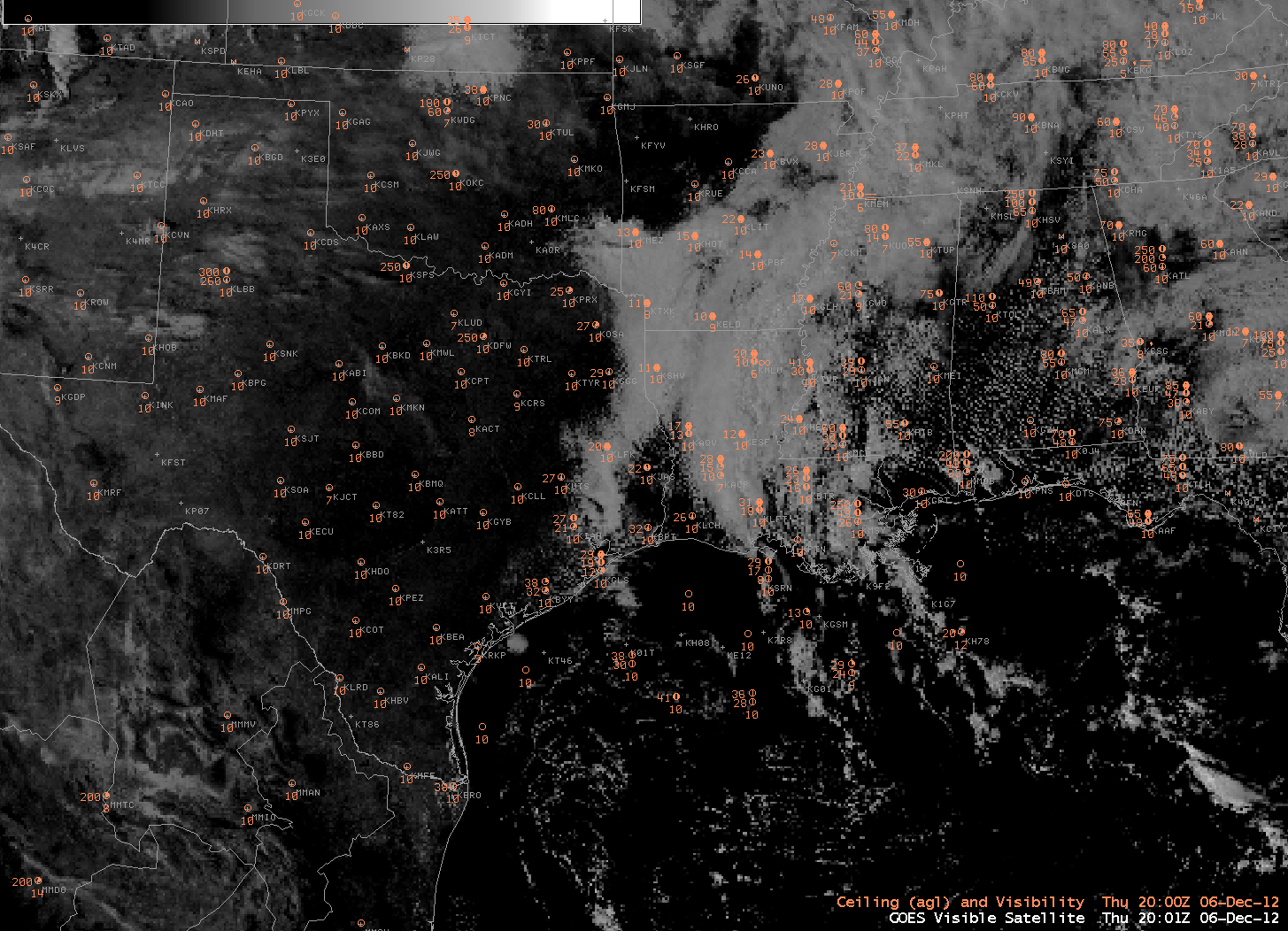
| Visible Imagery from 2000 UTC |
Visible imagery from 2000 UTC, above, shows that, although the fog has lifted, it has not burned off in 5 hours as predicted by the thickness/burn-off time relationship (here). This may be related to the very low sun angle in December.
(Added: This image loop shows how thin cirrus can show up in the brightness temperature difference product at night (this example is from Suomi/NPP even when fog-bound valleys are plainly evident in the Day/Night band at the same time!)


