Author Archives: Scott Lindstrom

Parallel Lines in IFR Probability over the Great Plains

GOES-R IFR Probabilities over the Great Plains. Notice the north-south lines/artifacts in the field over Kansas and Nebraska (Click to enlarge)

GOES-R IFR Probability fields over the Plains can sometimes include structures as shown above. These are related to the sloped topography of the Great Plains. They occur because of interpolation between model layers and the lowest 1000 feet that are examined for saturation. In a sloping region, quick changes in saturation amount can occur where changing topography changes which model levels are used in the examination of those lowest 1000 feet.

In other words, satellite pixels that are very close horizontally may nevertheless have different surface elevations that cause different profile levels to be analyzed for the maximum relative humidity (RH). If the RH drastically changes at the bottom or top of the profile being analyzed then differences will emerge as shown above. Extra interpolation before the profile is analyzed may mitigate this issue and could be incorporated into the algorithm in the future.

Resolution Matters

GOES-R IFR Probabilities computed from MODIS data and from GOES-15 data, ~1000 UTC on 22 June 2015 (Click to enlarge)

GOES-R IFR Probability was created with an eye towards using data from GOES-R (currently scheduled for launch at the end of March 2016). GOES-R will have better spatial, temporal and spectral resolution than the present GOES. A benefit of better spatial resolution is shown in the toggle above between present GOES (nominal 4-km resolution — vs. the nominal 2-km resolution that will be on GOES-R) and MODIS (1-km resolution). The small valleys along the northern California coastline are far better resolved. The fog/low clouds over San Francisco bay is also better resolved (and the same could be said for the Salinas Valley, south of Monterey Bay if this scene were shifted slightly south). (You might notice a slight 1-pixel shift between MODIS and GOES-15 IFR Probabilities. GOES-15 navigation is compromised by the lack of star-tracking data, so MODIS data are probably better navigated.)

GOES-15 Brightness Temperature Difference (10.7 µm – 3.9 µm) and GOES-R IFR Probabilities, 1000 UTC on 22 June 2015 (Click to enlarge)

IFR Probabilities are derived from GOES-15 brightness temperature difference fields, and a benefit of the IFR Probabilities is obvious above. Brightness Temperature Differences can be driven by emissivity differences in soil. These false positives over Nevada (from the point of view of fog detection) are easily removed if the Model Data does not show low-level saturation.

Suomi NPP Day/Night band imagery, Brightness Temperature Difference Fields (11.45 µm – 3.74 µm), and 3.74 µm Image, 0921 UTC on 22 June 2015 (Click to enlarge)

Suomi/NPP’s early morning overpass also detected the presence of fog/low stratus over the valleys along the northern California coast. The Brightness Temperature Difference field shows things distinctly. The Day-Night Visible imagery shows little in the way of fog on this day, as the waxing crescent moon had already set so no lunar illumination was present. The Day Night band is included here because it shows a very bright wildfire south of Lake Tahoe. That feature is also present in the 3.74 µm imagery. Fog and stratus is also evident in the 3.74 µm imagery, detectable based on its very smooth appearance.

IFR Conditions over eastern Massachusetts and the Cape

GOES-R IFR Probability, 0315 through 1215 UTC on 22 June 2015 (Click to enlarge)

Sea fog penetrated inland over eastern New England overnight. How did GOES-R IFR Probabilities depict the event, and how did those fields compare to the traditional fog-detection method, brightness temperature differences between the 10.7 µm and 3.9 µm channels? The animation above shows the IFR Probabilities, and they neatly outline the regions of low ceilings and reduced visibilities.

In contrast, Brightness Temperature Difference fields, shown below, are troubled by two different factors in these loops. Around 0700-0800 UTC, thin cirrus over southern Cape Cod impedes the satellite view of low clouds (Click here for a toggle between the two fields at 0722 UTC); brightness temperature difference fields yield little information when that happens. (GOES-R IFR Probability values drop when the Satellite component cannot be used; make certain when interpreting the values that you are aware of the presence/absence of high clouds!) In addition, the brightness temperature difference field loses features around sunrise, when solar radiation with a wavelength around 3.9 µm increases. GOES-R IFR Probability fields maintain a coherent signal through sunrise, however.

Careful inspection of the animation above does reveal some stations where IFR Conditions occur and IFR Probabilities are low. For example, Lebanon NH in the Connecticut River Valley reports IFR Conditions intermittently. Small-scale valley fog is a challenge for both GOES detection and for Rapid Refresh detection.

GOES-13 Brightness Temperature Difference Fields (10.7 µm – 3.9 µm), ~0315-1215 UTC on 22 June 2015 (Click to enlarge)

Dense Fog over eastern Maine

GOES-R IFR Probability Fields, hourly from 0315 to 1215 UTC on 10 June 2015 (Click to enlarge)

A cold front that moved across Maine early in the morning on 10 June 2015 was accompanied by dense fog. Dense Fog Advisories were hoisted over eastern Maine (screenshot from weather.gov; screenshot from the Caribou ME National Weather Service). The hourly imagery of IFR Probabilities, above, showed high probabilities over eastern Maine (where surface observations are scant). Note how the back edge of the high IFR Probabilities, after the frontal passage, correlates will with the timing of rising ceilings and reduced visibilities. This occurs at Augusta (KAUG), Bangor (KBGR) and Millinocket (KMLT), for example.

The traditional method of detecting fog and low cloud, the brightness temperature difference field that compares values at 10.7 µm and 3.9 µm , had difficulty indicating regions of fog for two reasons on the morning of 10 June. An animation of the product is below. There were high clouds present that interfered with the satellite’s view of low clouds. (IFR Probability can still give a useful signal in this case because of information that comes from the Rapid Refresh Model). In addition, the ever-earlier sunrise in early June supplies enough 3.9 µm radiation at the end of the animation to flip the sign of the brightness temperature difference field and the distinct signal of low water-based clouds is lost.

Brightness Temperature Difference Fields (10.7 µm – 3.9 µm), hourly from 0315 through 1215 UTC on 10 June 2015 (Click to enlarge)

Lead Time with GOES-R IFR Probabilities and Brightness Temperature Difference

A small region of dense fog developed over northeast Colorado and western Nebraska during the early morning on June 1st 2015. How did the GOES-R and traditional products handle this event? The animation below shows IFR Probabilities from 0730-0800 UTC on 1 June. Probabilities jump from <10% to about 20% at 0800 UTC in a region centered on Holyoke, CO, just south of I-76 in northeast Colorado. The Brightness Temperature Difference Field for the same 3 times, below the IFR Probabilities, shows a signal moving over the region but not substantially changing. (From this, one could conclude that the Rapid Refresh model data might be driving increase in the IFR Probability field)

GOES-R IFR Probabilities, 0730-0800 UTC on 1 June (Click to enlarge)

GOES-East Brightness Temperature Difference fields (10.7 µm – 3.9 µm) at 0730, 0745 and 0800 UTC, 1 June 2015 (Click to enlarge)

Toggle between GOES-R IFR Probabilities and GOES-East Brightness Temperature Difference Fields, 0915 UTC on 1 June (Click to enlarge)

By 0915 UTC (above), IFR Probabilities and GOES-13 Brightness Temperature Difference fields show a strong signal over NE Colorado where IFR Conditions occur/are developing. IFR Probability fields have provided more lead-time in the development of this region of low ceilings and visibilities. By 1100 UTC (below), a stronger, more widespread signal is apparent in both fields. At 1230 UTC (bottom), the rising sun has altered the brightness temperature field so it gives no useful information on low clouds; this highlights an advantage of GOES-R IFR Probability fields: A consistent signal through sunrise.

Toggle between GOES-R IFR Probabilities and GOES-East Brightness Temperature Difference Fields, 1100 UTC on 1 June (Click to enlarge)

Toggle between GOES-R IFR Probabilities and GOES-East Brightness Temperature Difference Fields, 1230 UTC on 1 June (Click to enlarge)

Fog over Coastal California

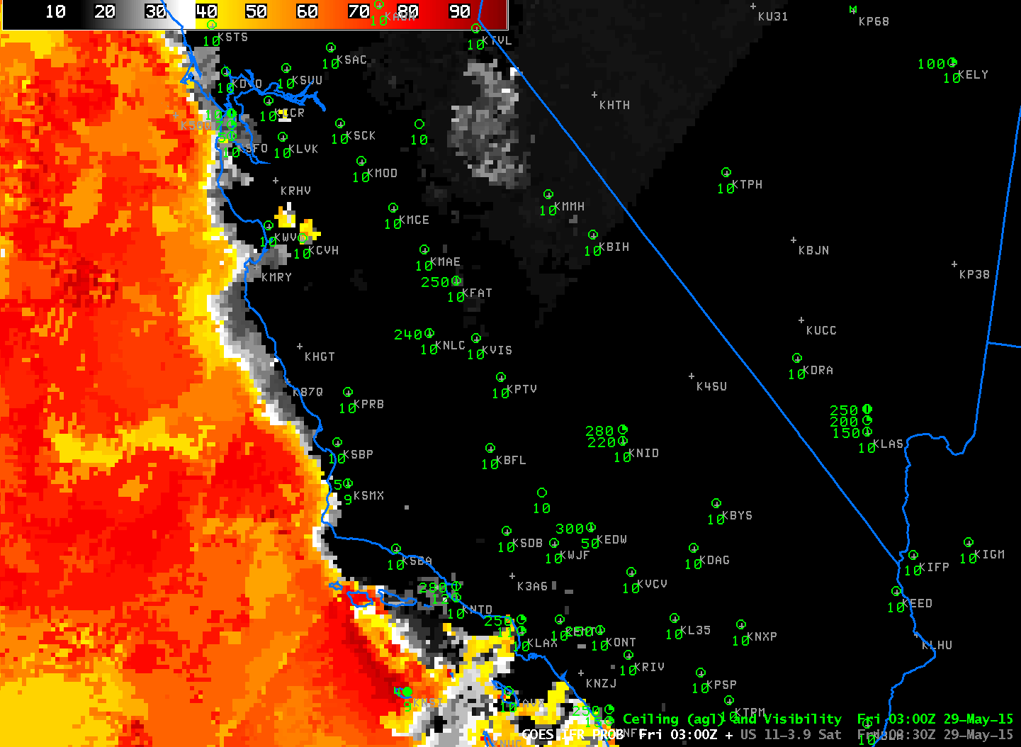
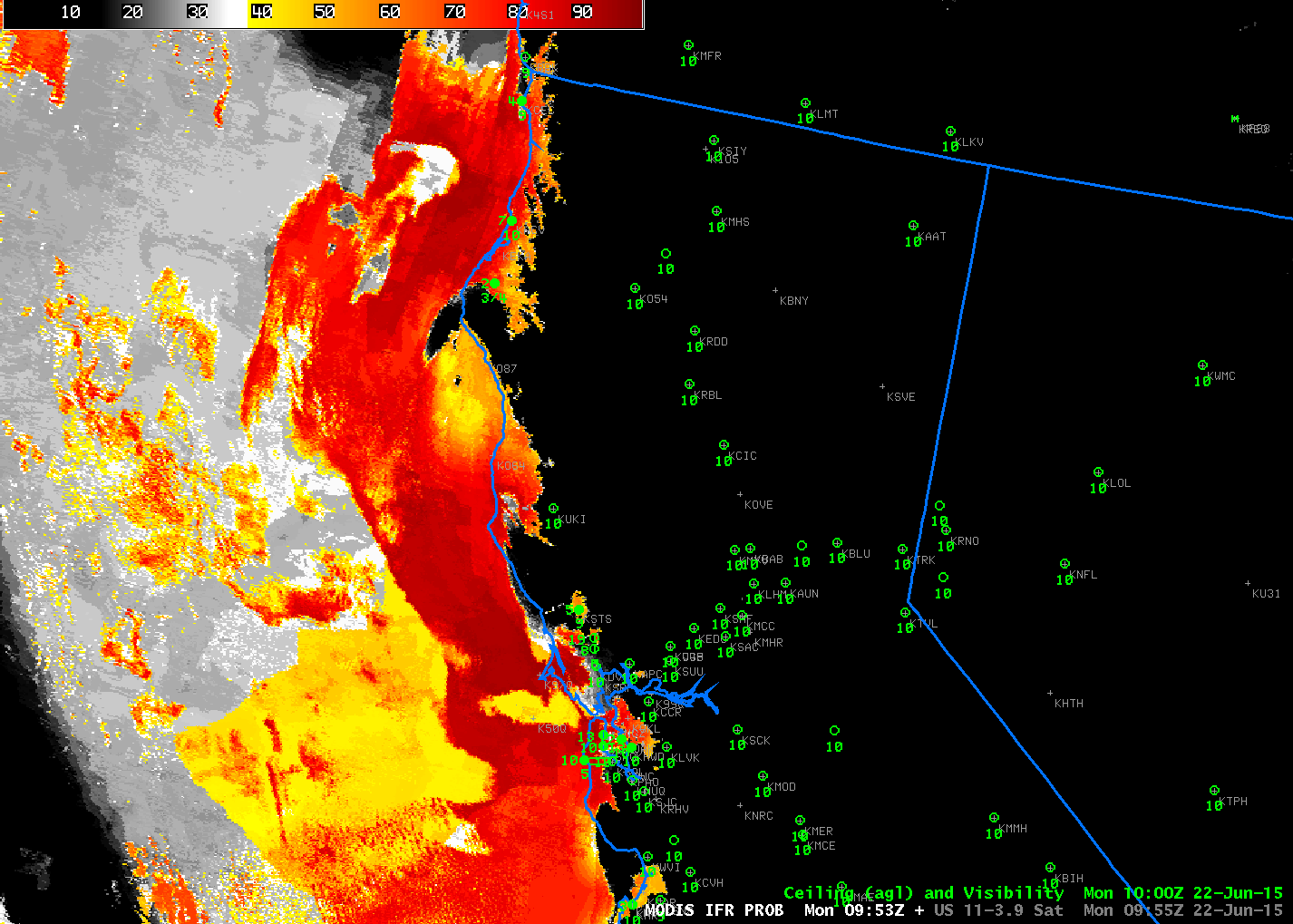
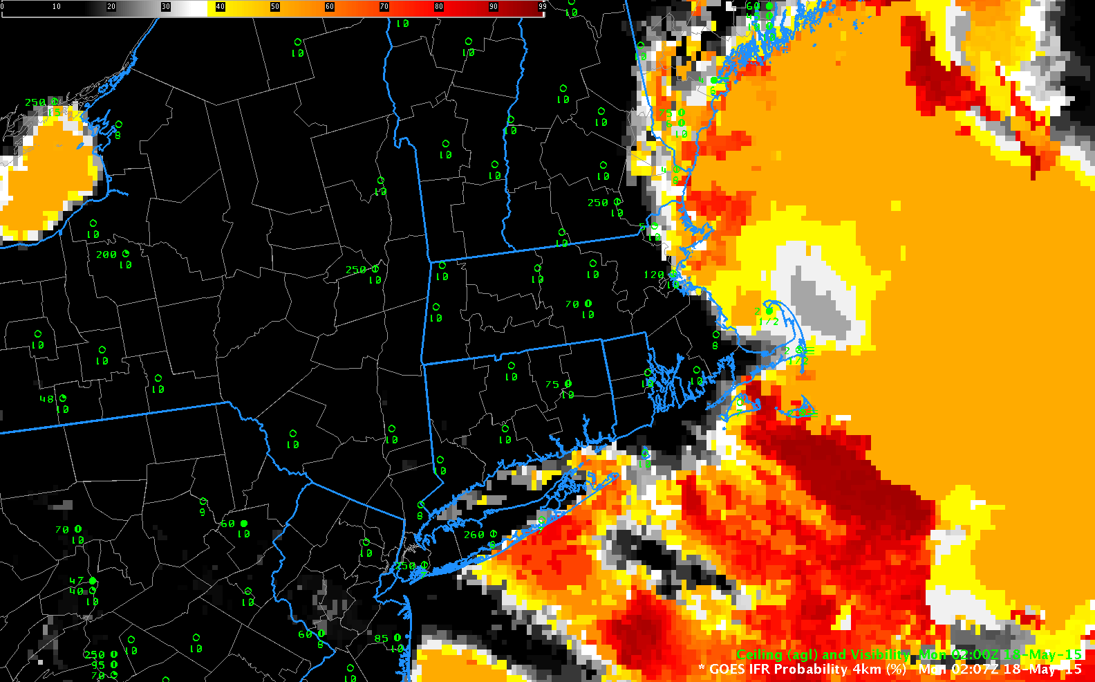
GOES-R IFR Probabilities computed from GOES-West and Rapid Refresh Data, 0300-1200 UTC on 29 May 2015 (Click to enlarge)

GOES-R IFR Probability fields are challenged most days by the diurnal penetration of coastal fog and stratus that occurs overnight along the California Coast. In the animation above, IFR Probabilities increase in regions along the coast, and also in valleys (such as the Salinas Valley) where fog moves inland. Note above how Monterey, Watsonville and Paso Robles all show IFR (or near-IFR) conditions as the IFR Probabilities increase. The same is true farther north at Santa Rosa and at Marin County Airport, and farther south at Avalon, Ontario, Point Mugu and LA International. IFR Probability fields routinely do capture these common fog events.

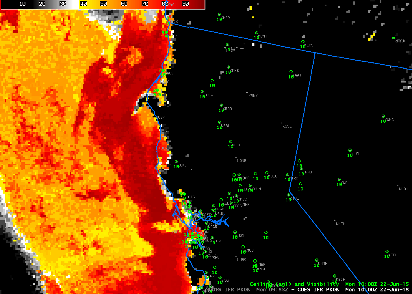
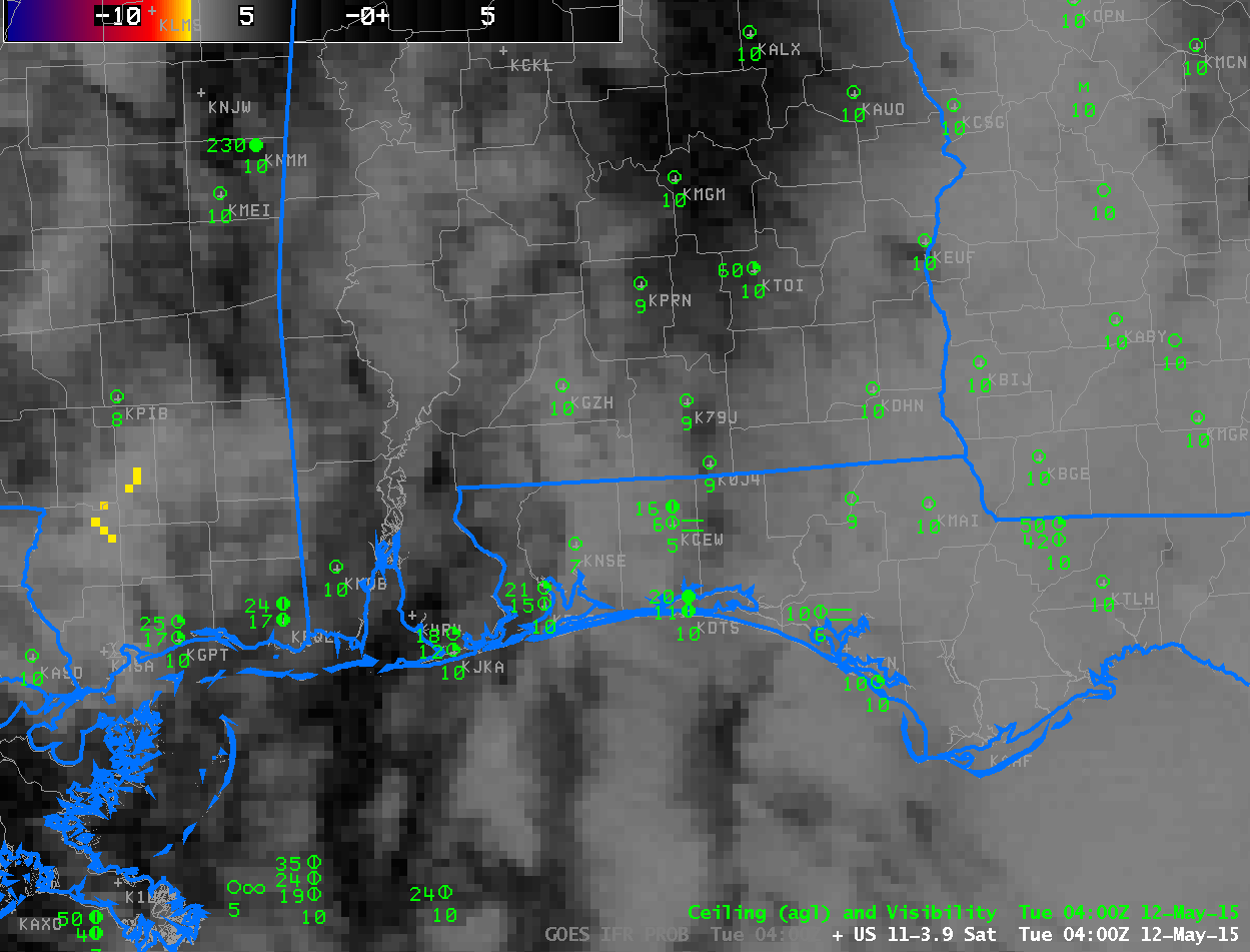
The Brightness Temperature Difference Field (10.7 µm – 3.9 µm), below, captures the motion of these low clouds as well. However, numerous ‘false positive’ signals occur over the central Valley of California (likely due to differences in soil emmissivities). The GOES-R IFR Probability field can screen these regions out because the Rapid Refresh data in the region does not show saturation in the lowest kilometer. Note also how the Brightness Temperature Difference field gives little information about low clouds where high clouds are present (over the Pacific Ocean in the images below). IFR Probability fields, however, do maintain a strong signal there because data from the Rapid Refresh strongly suggests the presence of low clouds/fog.

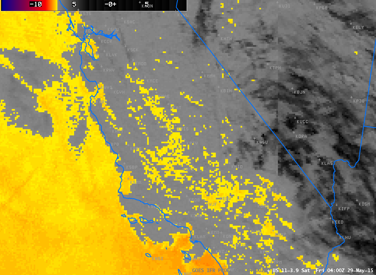
GOES Brightness Temperature Difference Fields, 0400-1200 UTC on 29 May 2015 (Click to enlarge)

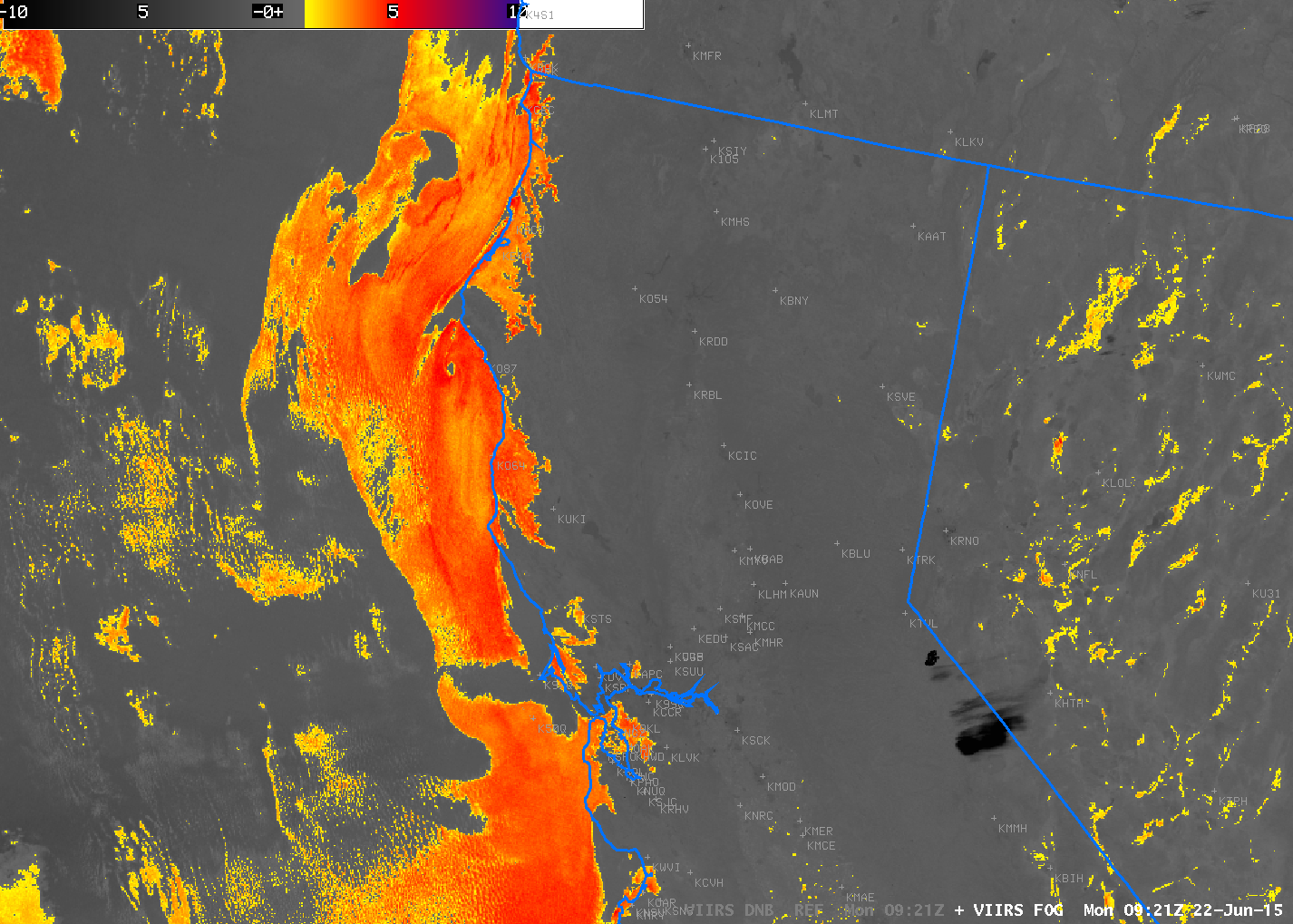
Suomi NPP makes an overflight over the West Coast each day around 1000 UTC, and the toggle of the Day Night Band and the Brightness Temperature Difference field (11.45 µm – 3.74 µm) is shown below. The moon at this time was below the horizon, so illumination of any fog is scant; the brightness temperature difference field does highlight regions of water-based clouds (that is, stratus); however, it does not contain information about the cloud base. In other words, it’s difficult to use the brightness temperature difference product alone to predict surface conditions.

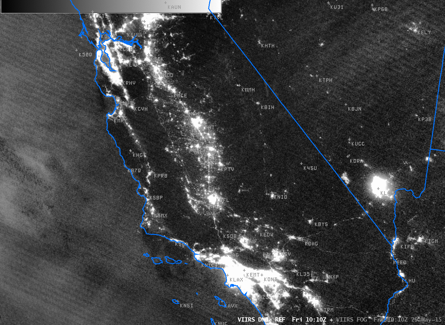
1010 UTC Imagery from Suomi NPP VIIRS Instrument: Day Night Visible Band (0.70µm) and Brightness Temperature Difference Field (11.45µm – 3.74µm) (Click to enlarge)

GOES-14 is in SRSO-R mode, and its view today includes the west coast. The animation below shows the erosion of the fog after sunrise at 1-minute intervals. (Click here for mp4, or view it on YouTube). (Click here for an animation centered on San Francisco).

GOES-14 Visible (0.6263 µm) animation, 29 May 2015 [click to play very very large animation]

Late Spring in the Great Lakes: Fog

GOES-R IFR Probability fields, 2100 UTC on 26 May 2015, along with surface observations of ceilings and visibility (Click to enlarge)

Sea or lake surface temperatures are part of the algorithm used to create IFR Probability fields. The cold Great Lakes in late May are a prime location for advection fog, and IFR Probability fields will blanket the Great Lakes with high values under southerly, moist flow. It is not uncommon to see all of the Lakes bright orange/red. Note in the image above how Manitowoc WI and Charlevoix MI both have IFR Conditions. In addition, Dense Fog advisories were issued north of Milwaukee to the tip of Door County.

Post-thunderstorm Fog over Mississippi

GOES-R IFR Probability Fields, ~hourly, from 0300 through 1200 UTC on 19 May 2015 (Click to enlarge)

Thunderstorms moved through Mississippi (See this animation — from this Blog Post — of SRSO-R 1-minute imagery from 18 May), and the low-level moisture left behind allowed Dense Fog to form, and Dense Fog advisories were issued.

Multiple cloud decks — shown in the toggle, below, of Suomi NPP Day Night Band and Brightness Temperature Difference (11.45 µm – 3.74 µm) — prevented the traditional brightness temperature difference product from providing useful information. GOES-R IFR Probabilities, shown ~hourly in an animation above do highlight the region of developing IFR conditions. Low ceilings and reduced visibilities are commonplace in regions where IFR Probabilities are increasing over night. The predictors that are included to compute the IFR Probabilities are mostly model-based because of the multiple cloud layers that are present, and the IFR Probability field is somewhat flat as a result. Note that GOES-R IFR probabilities increase at the very end of the animation; when daytime predictors are used, probabilities are a bit higher than when nighttime predictors are used.

Suomi NPP Day Night Band visible imagery and Brightness Temperature Difference (11.45 µm – 3.74 µm) at 0818 UTC, 19 May 2015 (Click to enlarge)

IFR Probabilities with a back-door cold front

GOES-R IFR Probabilities, hourly from 0200 through 1015 UTC on 18 May 2015 (click to enlarge)

Easterly winds south of a High over the Canadian Maritimes ushered in cool, moist air over the Northeastern United States early on Monday. IFR Probabilities, above, show the progress of the low ceilings and reduced visibilities that accompanied the change in air mass. The low clouds eventually penetrated to the Delaware River, as shown in the GOES-14 SRSO-R animation here (from this blog post).

In the animation above, observations of ceilings and visibilities over southern New England approach IFR conditions quickly as the IFR Probability ‘front’ passes through.

Fog in the Florida Panhandle

Dense Fog Advisories were issued for the northwestern part of the Florida Panhandle overnight (Link). How did various fog-alert satellite products perform for this case?

The brightness temperature difference product, below, that works because clouds comprising water droplets have different emissivity properties at 3.9 µm and 10.7 µm, did not provide much guidance for this event. This is because multiple cloud layers prevented the satellite from seeing down to the developing stratus/fog deck near the surface. The cloud deck persisted over Alabama, but eroded over northwest Florida by 0700 UTC. (Click here for an animation of GOES-Sounder Cloud Heights). In addition, fog persists through sunrise, and the rising sun is emitting 3.9 µm radiation; that makes interpretation of the brightness temperature difference field problematic.

Brightness Temperature Difference Fields (10.7 µm – 3.9 µm) from GOES East, ~hourly from 0400 through 1215 UTC on 12 May 2015 and surface observations of ceilings and visibilities (Click to enlarge)

The GOES-R IFR Probability field, below, provided better information about the developing cloud field. Probabilities increase as the fog develops, and the spatial coverage of the enhanced IFR Probabilities better matches the regions where Dense Fog Advisories were issued. In addition, the strong signal persists through sunrise.

GOES-R IFR Probability Fields computed from Rapid Refresh and GOES-13 Data, ~hourly from 0400 through 1215 UTC, and surface observations of ceilings and visibilities (Click to enlarge)

GOES-R Fog Product Examples

Fog detection fusing GOES, Terra/Aqua or Suomi/NPP Satellite data with Model output