Monthly Archives: December 2012

Predicting the dissipation time of Radiation Fog

GOES-R IFR Probabilities (Upper Left), GOES Brightness Temperature Difference (10.7 µm – 3.9 µm) (Upper Right), GOES-R Cloud Thickness (Lower Left), GOES Visible (0.62 µm) (Lower Right) at 1400 UTC on 27 December 2012.

GOES-R Cloud thickness can be used to predict how long it will take radiation fog and low stratus to burn off after developing overnight.  This case from the high plains of Colorado, on December 27th, is typical.  At 1402 UTC, La Junta Colorado is in a region of enhanced IFR Probability, with 2-mile visibilty and 400-foot ceilings.  The Cloud Thickness at this time, the last image available before twilight conditions, was as much as 1200 feet.  This scatterplot suggests that the fog will be gone in 4-5 hours.  The 1732 UTC image, below, shows the final remnant of low cloud persisting (it was not present at 1815 UTC).  Although difficult to see in the visible imagery, perhaps because of snow-covered ground, it shows up well in both the IFR probability field, the Brightness Temperature Difference field, and the Cloud Thickness field.

As above, but at 1732 UTC.

Interpreting IFR Probabilities when multiple Cloud Layers exist

GOES-R IFR Probabilities computed from GOES-East and the Rapid Refresh, 1400 UTC 26 December 2012, and surface observations of ceilings and visibilities.

Large winter-time extratropical storms generate multiple cloud layers, and those many layers make difficult the detection of IFR conditions at the surface, caused by fog and low stratus.  The winter storm moving up the East Coast on December 26th, 2012, is typical of the type of storm that causes these conditions (although its abnormal production of tornadoes is very atypical).  In the figure above, IFR probabilities are high over eastern North Carolina, and those high probabilities are generated solely from Model Data.  Satellite information from GOES-East there is not useful because of multiple cloud layers.  There are regions over western North Carolina — where the GOES-R IFR probability field is less smooth and more pixelated — where GOES data indicate low-level clouds only and both satellite data and model data contribute to the IFR Probability fields.

GOES-R IFR Probabilities (Upper Left), GOES-East Brightness Temperature Difference Field (10.7 µm – 3.9 µm ) (Upper Right), GOES-R Cloud Thickness (Lower Left), GOES-East Visible Imagery (0.62 µm) (Lower Right)

The hourly animation of GOES-R IFR probabilities, Traditional Brightness Temperature Difference, GOES-R Cloud Thickness and Visible Imagery, above, is instructive on several points.  The Traditional Brightness Temperature Difference, because of the abundant high clouds (likely associated with the warm conveyor belt of the extratropical storm), yields little information about low-level conditions.  Note also how Cloud Thickness field is computed in one region:  the region where multiple cloud layers do not exist, and where twilight conditions are not present.  There are also differences in the GOES-R IFR Probability field between day and night that reflect the different predictors (and different predictor weights) that are used during those two times.

From the Archives: December 3, 2012

It is always possible to reconstruct the GOES-R IFR Products and to re-inject them into AWIPS for case studies.  For example, Columbia, SC, notified us of a fog event there on the morning of December 3rd, 2012 (See here).  The imagery below was created on 19 December and shows the development of the GOES-R IFR probabilities over the entire southeast during this event.

GOES-R IFR Probabilities from 3 December 2012

IFR probabilities increase first along coastal South Carolina and Georgia and then increase inland.  The animations below show the hourly changes in visibility (top) and ceiling (bottom) from 0000 UTC to 1400 UTC on 3 December.

Visibility (Statute Miles) from 0000 UTC to 1400 UTC on 3 December

Ceiling Height (feet) from 0000 UTC to 1400 UTC on 3 December 2012

The brightness temperature difference animation, below, from 0145 UTC through 1345 UTC, shows the development of the low stratus over coastal South Carolina and Georgia.  The Brightness temperature difference field loses its signal at sunrise, however, even though observations show fog and low stratus persisting.

Brightness Temperature Difference (BTD) (10.7 µm – 3.9 µm) from 0145 UTC through 1345 UTC, from GOES-East

IFR Conditions during a Weak weather event

GOES-East Water Vapor Imagery (6.7 ) from 2202 UTC on 18 December 2012

A weak weather system moved through the upper Midwest on December 18th, laying down a light strip of snow over Iowa and southern Wisconsin.  The Water Vapor imagery, above, shows the small scale vorticity center that helped to force the precipitation band moving over southern Lake Michigan after most of the snow in Wisconsin had tapered off.

The storm left behind abundant low-level moisture, and Fog/Low Stratus that caused IFR conditions were common.  The animation of the GOES-R IFR Probability product, below, shows high probabilities in the region where light snow and drizzle persisted.  Several aspects of this image require comment.

GOES-R IFR probabiltiies computed from GOES-East, and surface observations of ceilings and visibility, hourly from 2100 UTC 18 December to 0200 UTC 19 December.

The image at 2200 UTC shows the boundary between day-time predictor use and night-time predictor use.  This boundary runs southeast to northwest over Iowa.  IFR probabilities are somewhat lower where the night-time predictors are used initially, but patches of higher IFR probability do occur.  The IFR Probability product does distinguish well between the fog and low stratus that does restrict visibility and the elevated stratus over Illinois that is obvious in the traditional brightness temperature difference product, below.  Note especially how Chicago’s O’Hare airport is not reporting IFR conditions, nor under a region where GOES-R IFR probabilities are high, but it is in a region where the traditional brightness temperature product has a strong signal.

Toggle between GOES-R IFR Probability field and GOES-East Brightness Temperature Difference Field, 0200 UTC 19 December 2012

Know your Terrain!

GOES-R IFR Probabilities (Upper left), GOES Brightness Temperature Difference (10.7 – 3.9 ) (Upper Right), color-enhanced Topography (Lower Left), Window Channel Infrared (10.7 ) (Lower Right).  Imagery from 0715, 1015 and 1415 UTC 18 December 2012.

Interpretation of the GOES-R IFR probability must include a consideration of terrain height, because a cloud bank that exists over a valley as elevated stratus can quickly become fog or low stratus as the ground rises into the fog on the sides of the valleys.  This happens with some frequency over the Sierra Nevada next to California’s San Joaquin valley, but it is also apparent in the images above over the higher terrain of central Idaho near the Snake River Valley.  A strong IFR Probability signal develops over central Idaho and also over eastern Idaho/northwest Wyoming where high terrain exists.

IFR conditions under high clouds in the Northeast

GOES-R IFR Probabilities computed using GOES-East (Upper Left), GOES-East Brightness Temperature Difference (10.7 µm- 3.9 µm, The ‘traditional’ fog detection product) (Upper Right), GOES-R Cloud Thickness computed using GOES-East (Lower Left), GOES-East Window Channel (10.7 µm) Brightness Temperature (Lower Right)

When high clouds overspread an area, the traditional brightness temperature difference product cannot be used to highlight areas of fog and low stratus because radiation emissions are originating from high clouds, not from the water-based low clouds.  In this example from Monday morning, 17 December 2012, IFR conditions, causing airport flight delays, are commons from Washington DC to New York, and the GOES-R IFR probability product highlights the area where IFR (and near-IFR) conditions prevail.  Modest values (around 50%) occur where the satellite predictors do not provide a fog/low stratus signal;  however, the Rapid Refresh model data does show high probability of fog and low stratus.  Where the Satellite does contribute to the product (that is, in Pennsylvania north and east of the high cloud deck), IFR probabilities are very high.

Note also that the GOES-R Cloud Thickness product (bottom left), is computed only for the highest water-based cloud (in non-twilight conditions).  It is therefore not shown under the cirrus canopy, over southern New Jersey, Delaware, and Chesapeake Bay.

Florida Radiation Fog

GOES-R IFR Probabilities (Upper Left) computed from GOES-East, GOES-East Brightness Temperature Differences (10.7 µm – 3.9 µm) (Upper right), GOES-R Cloud Thickness product (Lower Left), GOES-East Visible Imagery (0.63 µm) (Lower Right), hourly from 0615 UTC through 1215 UTC on 14 December 2012

Light north winds over Florida over night were accompanied by the development of low stratus and fog that were captured well by the traditional fog detection product, the brightness temperature difference between 10.7 µm and 3.9 µm that occurs because of emissivity differences in water clouds at the two wavelengths.  Because of the strong satellite signal (upper right), the GOES-R IFR Probabilities over Florida were quite high.  When mid-level and high clouds are absent, IFR probabilities in regions of fog development can easily exceed 90%, as shown above.

Note, however, what happens at sunrise.  The increase in reflected 3.9 µm solar radiation causes the brightness temperature signal to vanish.  (At later times, the sign of the brightness temperature difference will flip).  The GOES-R IFR probability product maintains a coherent signal through sunrise, although values shift somewhat, as can be seen by the southwest to northeast boundary in the final image of the loop over Florida and extreme southeast Georgia.

Cloud thickness, bottom left, can be used to estimate when radiation-induced stratus or fog will ‘burn off’ — thicker clouds will take longer to dissipate.

Note in this loop that the eastern coastline of Mobile Bay shows a signal in the Brightness Temperature Difference.  This signal is likely an artifact of poor co-registration between Bands 2 and 4 (the 3.9 µm and 10.7 µm channels, respectively) on GOES-13.  NESDIS scientists and engineers are working to mitigate this time-dependent error.

The Fog/Low Stratus products can be compared to data from Suomi/NPP.  The VIIRS instrument includes a day/night band that uses reflected moonlight as a light source (below).  Unfortunately, because the moon was new on December 13th, 2012, very little reflected light is available.  Nevertheless, smearing of city lights over Florida does suggest the presence of fog.

As above, but with Day/Night band from VIIRS on Suomi/NPP instead of GOES-13 0.63 µm visible imagery.  Images from ~0630 UTC on 14 December.

Fog Detection under multiple cloud layers

GOES-R IFR Probabilities computed from GOES-East data (Upper left), GOES-East traditional brightness temperature difference product (Upper right), GOES-East 10.7 µm imagery (Lower left), Surface observations of ceiling/visibility (Lower right)

Weather over Florida on 12 December 2012 gives another example of the importance of fused data products in computing IFR probabilities/detecting low clouds and fog.  When mulitple cloud layers are present, as today over Florida, the traditional brightness temperature difference product (10.7  µm – 3.9 µm) can struggle to produce a useful signal.  Adding information about the lowest part of the atmosphere from the Rapid Refresh model, however, allows a coherent prediction of IFR probabilities to be made.  Note that the stations with the most significant reductions in ceilings/visibility do align with the stripe of higher IFR probability over the northern part of the Florida peninsula.

Gulf of Mexico Fog

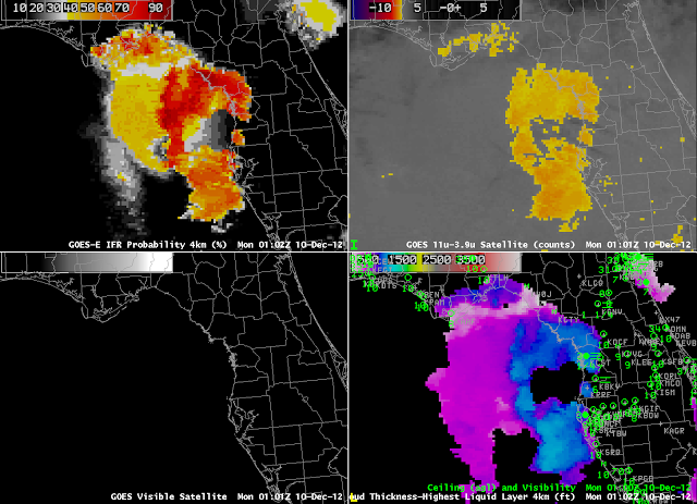
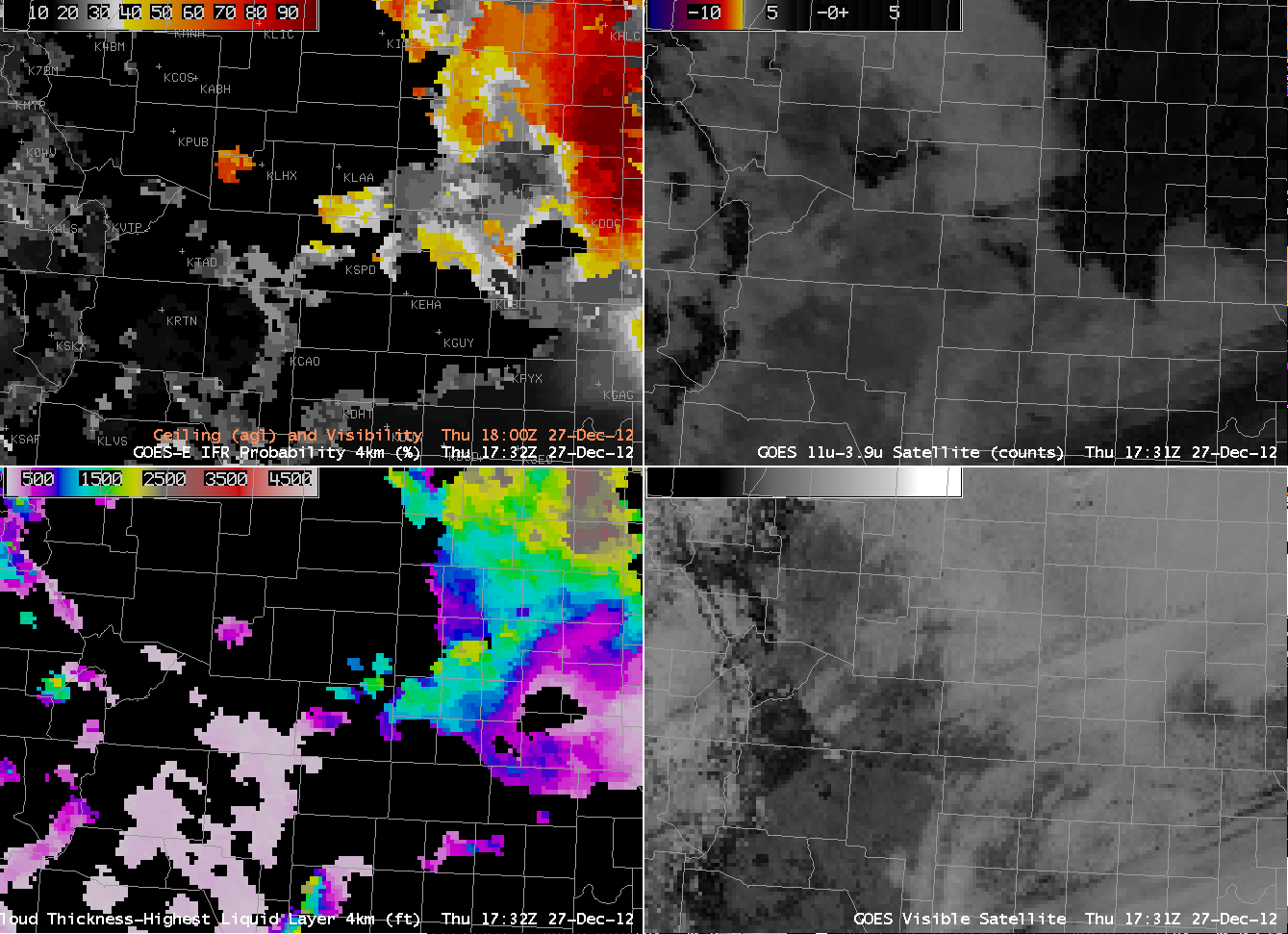
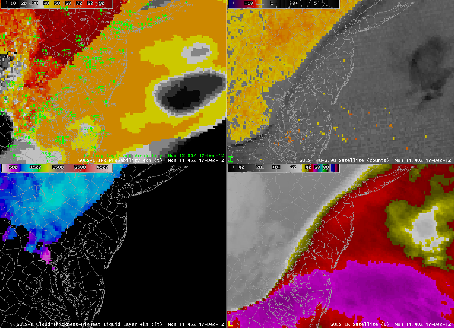
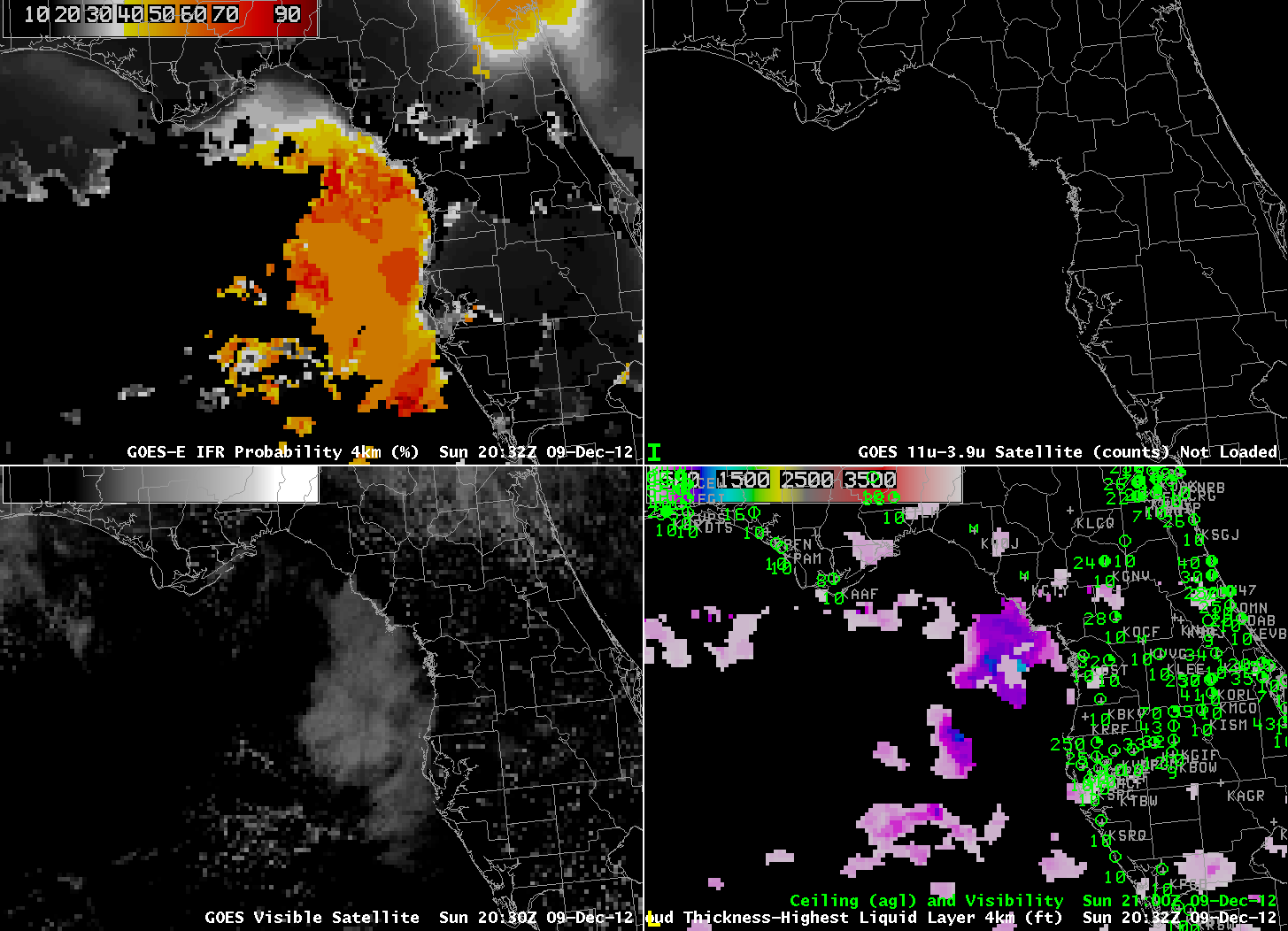
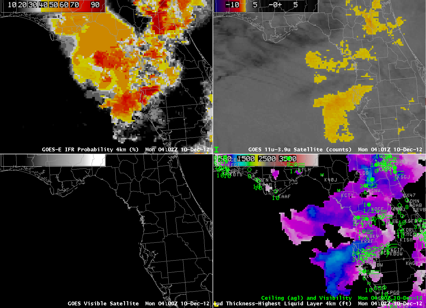
GOES-R IFR Probabilities computed from GOES-East (Upper Left), GOES-East Brightness Temperature Difference (10.7 µm – 3.9µm ) (Upper Right), GOES-East Visible imagery (0.63 µm) (Lower Left), GOES-R Cloud Thickness (Lower Right), all from ~2030 UTC on 9 December 2012

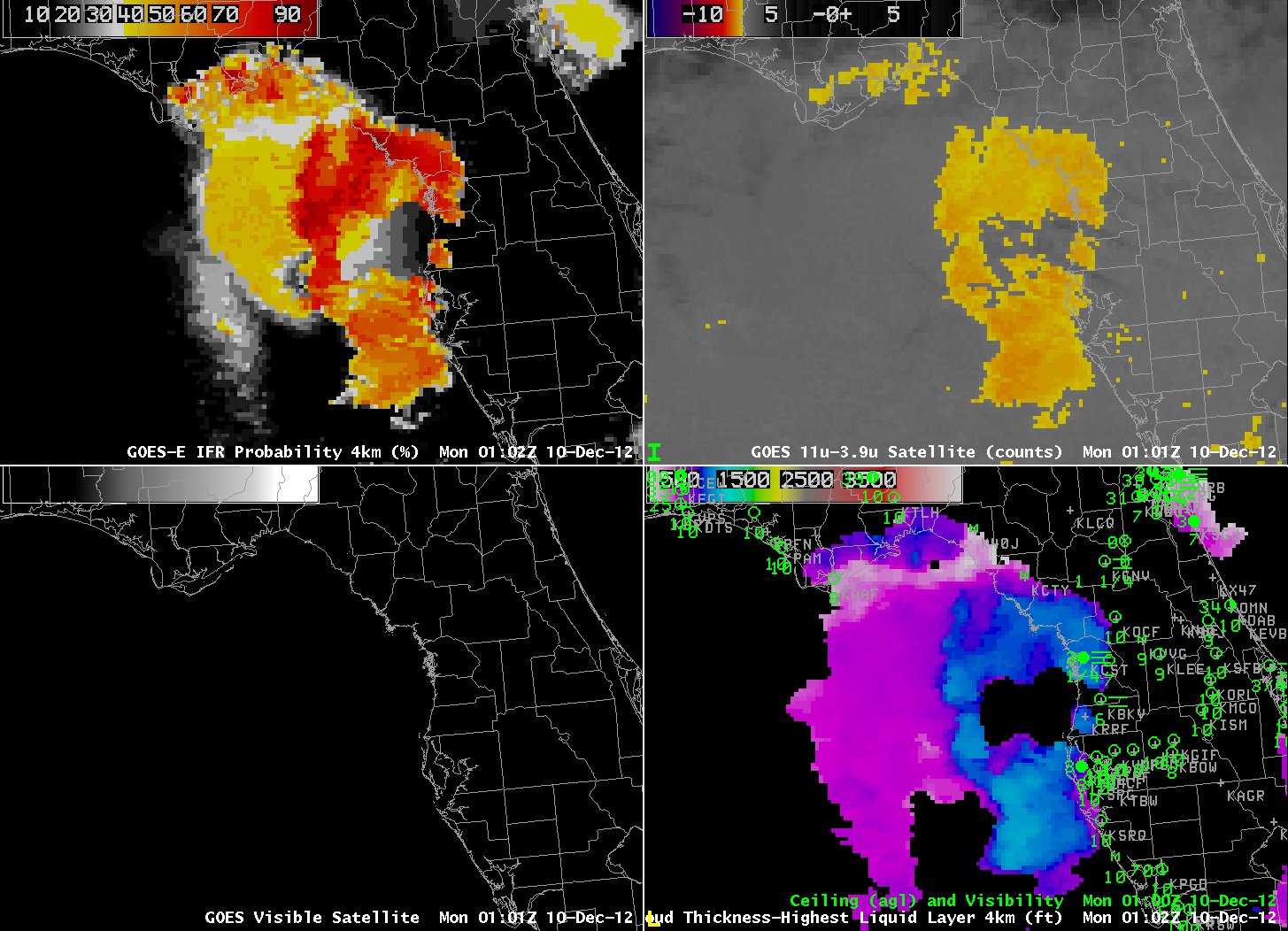
Fog was present in the northeast Gulf of Mexico at sunset on December 9th, and the GOES-R Products was able to track its evolution as it slowly moved onshore.  Late-in-the-day visible imagery from 2030 UTC 9 December (above) shows the fog bank tucked into the northeast corner of the Gulf of Mexico.  By 0100 UTC on 10 December (below), some of the fog as moved inland, and visibilities/ceilings at Crystal River have decreased to IFR conditions.  Note in the 0100 UTC image the presence of mid-level clouds is creating a hole in the Brightness Temperature Difference Signal over the eastern Gulf of Mexico just northwest of Tampa, and in the Cloud Thickness product.  IFR Probabilities in this region are considerably reduced, as well.

As at top, but for 0100 UTC on 10 December
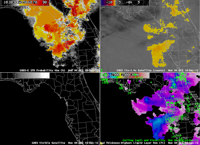
As above but for 0402 UTC on 10 December

By 0400 UTC on 10 December, the fog/low stratus continue to press inland, as ceilings and visibilities decrease.  Note also the presence of higher clouds in the brightness temperature difference product.  In these regions, satellite predictors are not use to compute the IFR probability product;  consequently, IFR Probabilities over and around Apalachee Bay in the extreme northeast Gulf of Mexico are somewhat reduced; in addition, the field is considerably flatter (compared to the more pixelated character close to Tampa).  At 0802 UTC (below), the presence of mid-level clouds peaks.  Note that the brightness temperature difference product shows very little strong signal over the northern part of the Florida peninsula, despite significant visibility obscurations there (consider Gainesville, for example, with a 1/4-mile visibility).

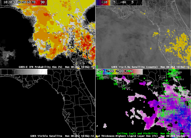
As above but for 0802 UTC on 10 December
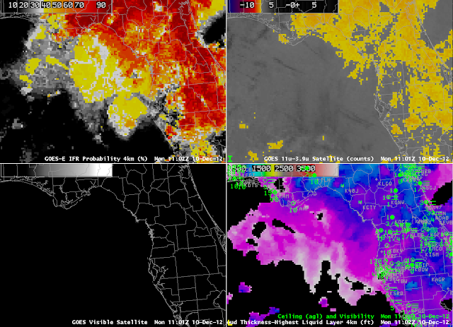
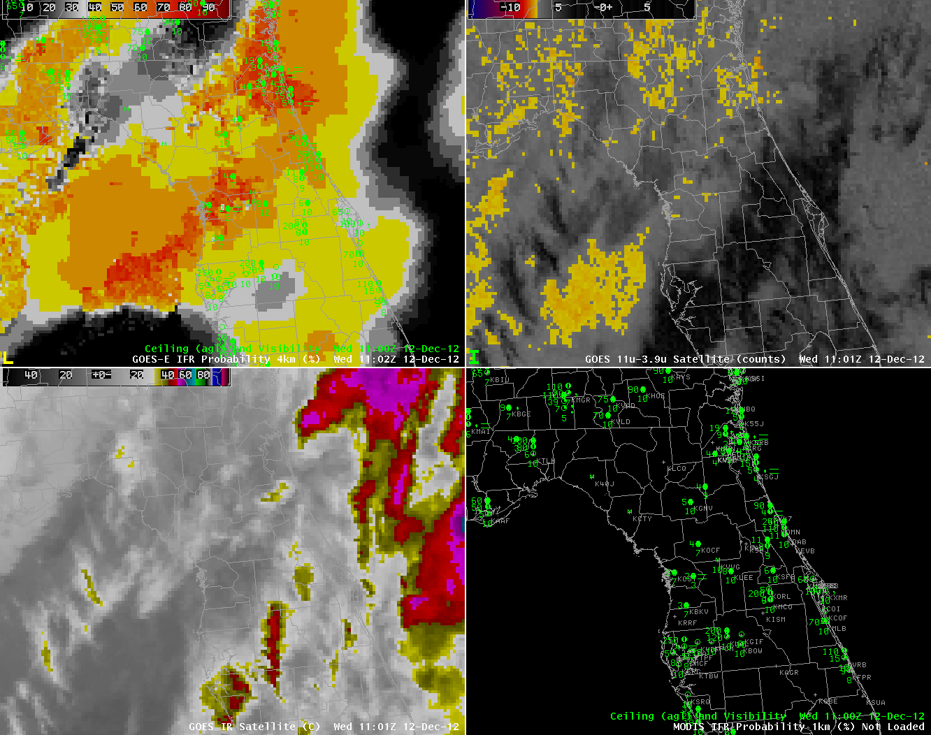
As above, but for 1102 UTC on 10 December

By 1102 UTC, the mid-level cloudiness has dissipated, allowing the brightness temperature difference to have a distinct signal.  Consequently, the IFR probability field increases.  The combination of both satellite predictors and model (Rapid Refresh) predictors being used allows for a consistent signal throughout the night over this evolving fog/stratus deck.  In addition, the signal over the ocean, at the end of the day on 9 December, in a region where surface observations are not routine, could serve as an alert to the early development of nocturnal fog.

Note that the Tampa Bay office of the National Weather Service noted the IFR probability field in its forecast discussion:

 
000
FXUS62 KTBW 100034
AFDTBW

AREA FORECAST DISCUSSION
NATIONAL WEATHER SERVICE TAMPA BAY RUSKIN FL
734 PM EST SUN DEC 9 2012

.FOR THE EVENING UPDATE...
SURFACE HIGH PRESSURE WILL REMAIN OVER THE REGION WITH A STRONG
MID LEVEL SUBSIDENCE INVERSION AND STABLE AIR MASS OVER THE
FORECAST AREA. AREA OF FOG...LOCALLY DENSE...HAS PERSISTED THROUGH
THE DAY OVER THE COASTAL WATERS NORTH OF VENICE AND LOCALLY
ONSHORE FROM ABOUT ANNA MARIA ISLAND NORTH TO CEDAR KEY. AREA OF
LOCALLY DENSE FOG WILL GRADUALLY PUSH ONSHORE THE COASTAL
COUNTIES THIS EVENING...WITH FOG DEVELOPING OVER INTERIOR BECOMING
LOCALLY DENSE AFTER MIDNIGHT. CURRENT ZONES ARE ON TRACK WITH NO
UPDATE PLANNED.

&&

.AVIATION...
GOES-R IFR AND LIFR PROBABILITY PRODUCTS NICELY OUTLINE AN AREA OF
SEA FOG THAT HAS LINGERED ACROSS NEAR SHORE WATERS FROM BIG BEND
SOUTH TO AROUND VENICE. THIS SEA FOG IS RIGHT ALONG THE COASTLINE
AND IS VISIBLE ON SOME BEACH WEB CAMS IN THE AREA AND THEREFORE IS
POISED TO MOVE INLAND ONCE TEMPS FALL SOME. THE BIG QUESTION IN ALL
THIS IS WHETHER THE WEAK WRLY WINDS ASSOC W/ THE SEA BREEZE
CIRCULATION WILL CONTINUE LATE ENOUGH TO PUSH THE SEA FOG BANK
INLAND IMPACTING TAMPA BAY AREA SITES. PREVIOUS TAFS WERE COUNTING
ON THIS OCCURRING AND WILL CONTINUE CLOSE TO THE FORECAST ALTHOUGH
HAVE NOTED 18Z MAV AND LATEST LAMP HAVE STRONGLY BACKED OFF ON THE
FOG FOG FORECAST AND NOW CONFINED FOG TO MUCH LATER IN THE NIGHT
CLOSER TO SUNRISE. WILL HAVE TO WATCH CLOSE AND AMEND AS NEEDED IN
NEXT FEW HOURS AS ONSET OF LIFR CONDITIONS IS BIGGEST QUESTION MARK
TONIGHT. LIFR CONDITIONS ARE PRETTY CERTAIN AROUND 12Z AND WILL SEE
SLOW IMPROVEMENT TO MVFR LEVELS THROUGH 18Z. MVFR LEVELS MAY LINGER
AND CONTINUE BEYOND 18Z AS MOISTURE SURGES INTO THE AREA LEADING TO
SCT SHRA ACROSS THE ENTIRE AREA AND POSSIBLY A FEW TSTMS MAINLY
AROUND OR EAST OF SRN SITES (FMY, RSW, PGD). MODELS SUGGEST
POTENTIAL DEVELOPMENT OF MORE WIDESPREAD SEAFOG EVENT LATE TOMORROW
AS MOISTURE CONTINUES TO INCREASE AND A MORE PERSISTENT SW FLOW
DEVELOPS. 
 
 
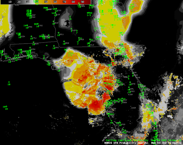
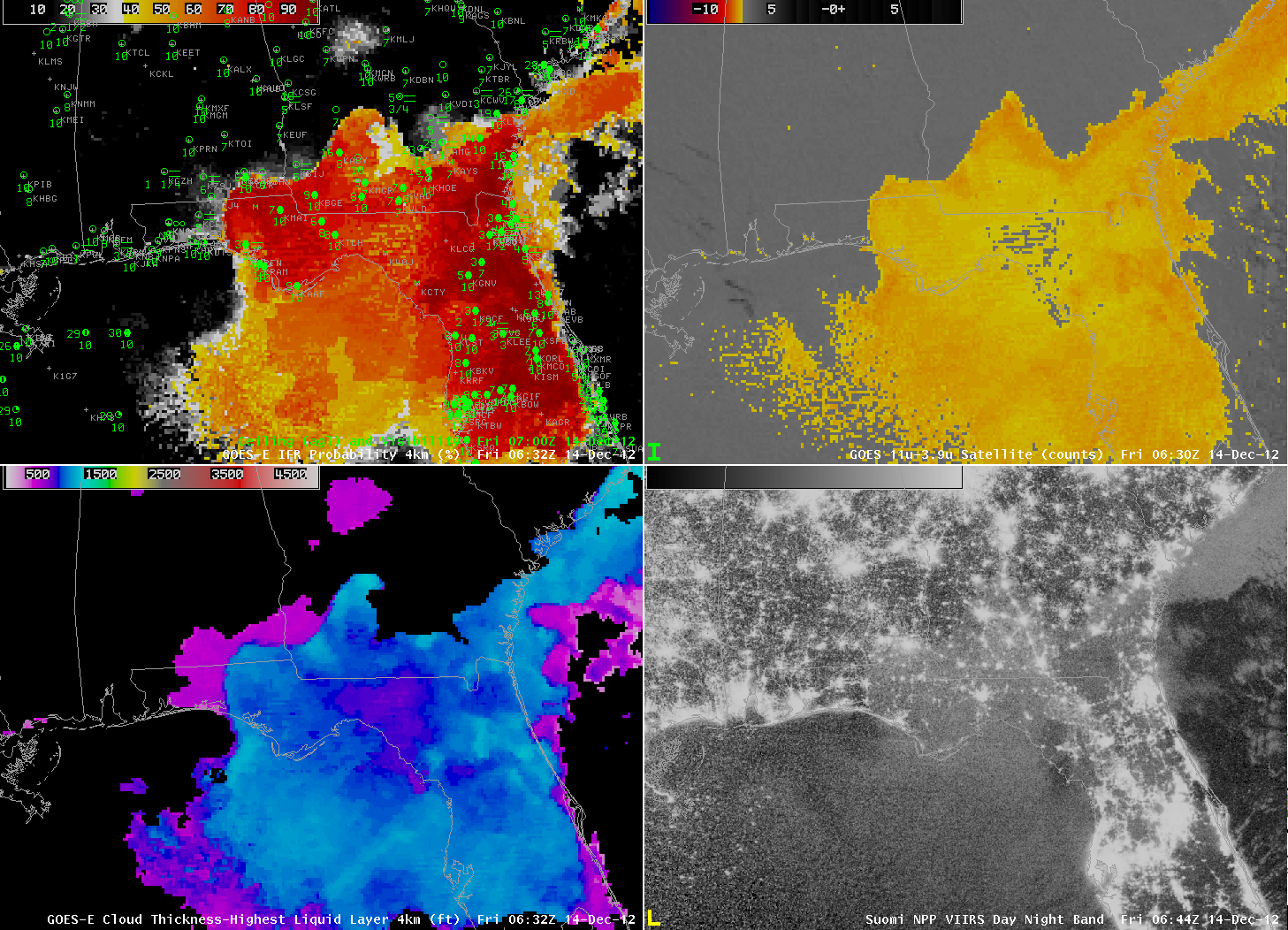
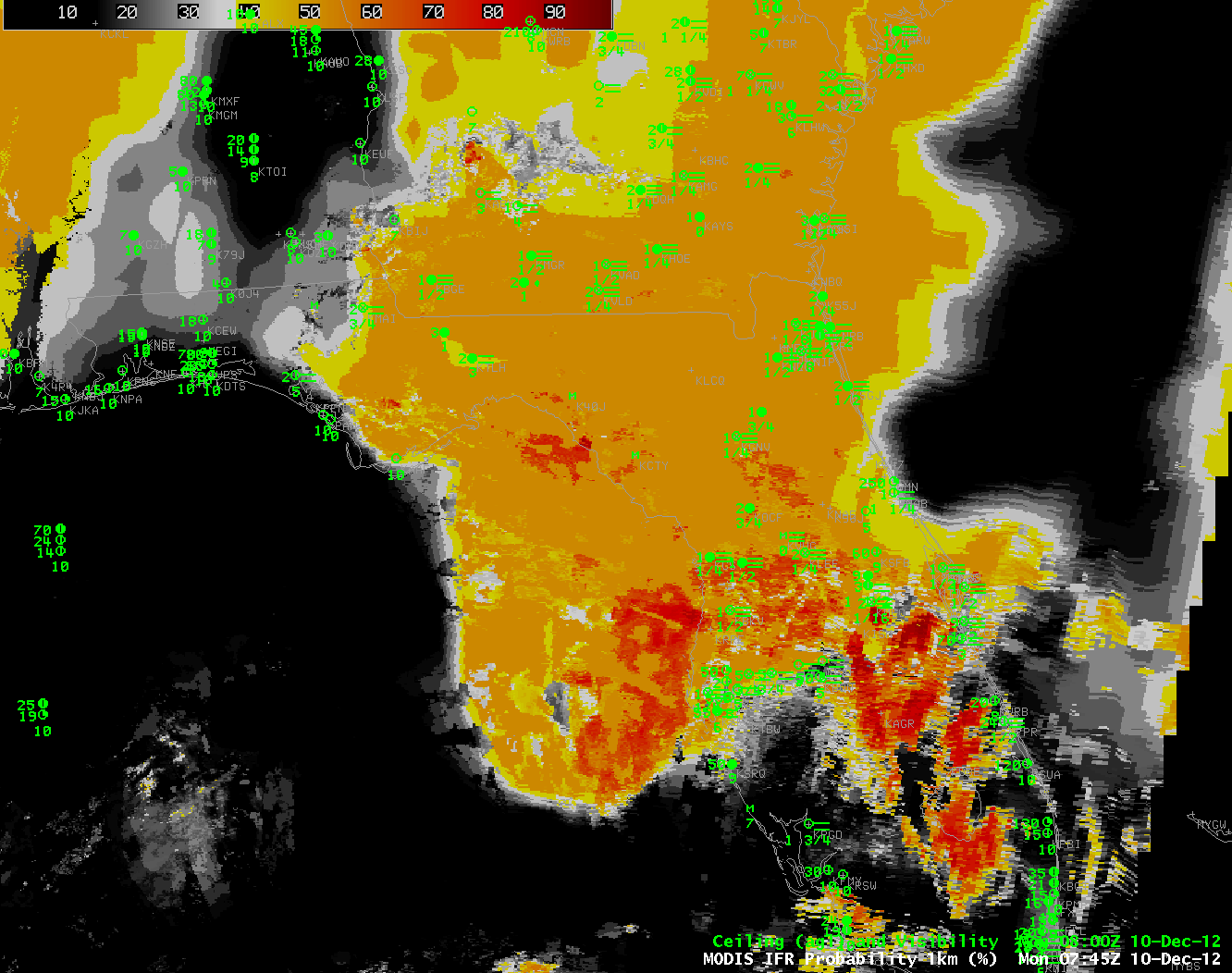
MODIS-based GOES-R IFR Probabilities, 0334 UTC 10 December (above) and 0745 UTC 10 December (below)

MODIS-based GOES-R IFR Probabilities, above, show a similar evolution of the field, from fairly constrained over northern Florida at 0334 UTC, and determined by both satellite and model fields, to more widespread but deteremined more by model fields only at 0745 UTC.

Fog in California’s San Joaquin Valley

GOES-R IFR Probabilities, computed from GOES-West (Upper Left), GOES-West Visible Imagery (0.62 µm) (Upper Right), GOES-R Cloud Thickness (Lower Left), GOES-West Brightness Temperature Difference (10.7 µm – 3.9 µm) (Lower Right)

Fog is persisting in California’s San Joaquin Valley today, and the GOES-R IFR Probability and Cloud Thickness products both are describing its spatial extent.  The lowest clouds are banked against the western side of the valley, with visibilities lowest, and IFR probabilities highest, from Bakersfield to Fresno to points north.  The Sacramento Valley (not shown) is not showing visibilities near IFR conditions, and the IFR probabilities in that part of California are lower.