GOES-16 IFR Probabilities (and surface observations of ceilings and visibilities), upper left ; GOES-16 Cloud Thickness, upper right ; GOES-16 ‘Night Fog’ Brightness Temperature Difference (10.3 µm – 3.9 µm), lower left; GOES-16 Nighttime Microphysics RGB, lower right. All from 0701 – 1301 UTC on 15 July 2021 (Click to enlarge)
The animation above shows various methods typically used to detect fog/low stratus in the early morning. Night Fog Brightness Temperature differences, bottom left, and Night Time microphysics, bottom right, are both satellite-only detection systems; a shortcoming might be that satellite data is challenged in detecting cloud bases — satellites view the cloud top. Additionally, the signal is lost as the sun rises. IFR Probability (upper right) includes information (from the Rapid Refresh model) on low-level saturation, so perhaps that field better defines the scattered pockets of fog apparent on this morning. However, the Rapid Refresh model resolution is 13-km, and a valley fog might not be well-resolved in the model.
The Cloud Thickness information suggests that any clouds are thin, and that morning burn-off will be speedy. That is indeed what happened, as shown by the 1500 UTC image below (taken from the CSPP Geosphere site). Recall that the Cloud Thickness product is not produced in the times that surround sunrise (or sunset).
CSPP Geosphere True Color image, 1500 UTC 15 July 2021 (Click to enlarge)
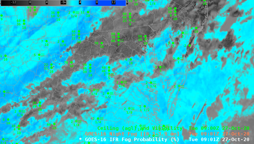
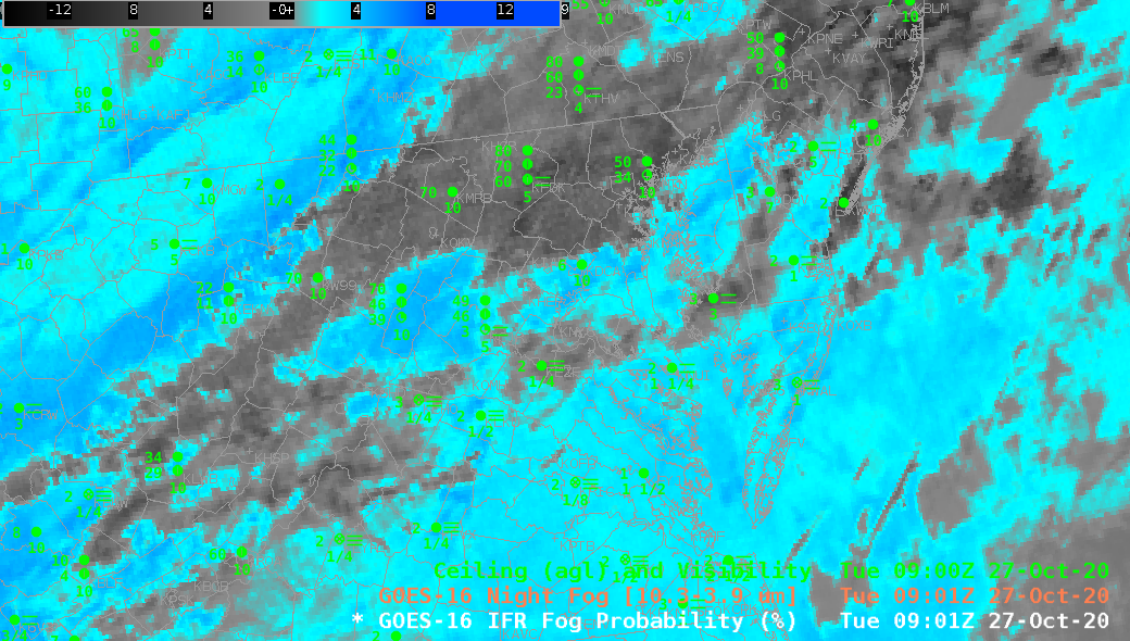
GOES-16 Night Fog Brightness Temperature Difference (10.3 µm – 3.9 µm) and IFR Probability at 0901 UTC, along with 0900 UTC plots of surface ceilings and visibility (Click to enlarge)
GOES-16 IFR Probability fields, above, from 0901 UTC on 27 October 2020 (in a toggle with the Night Fog Brightness Temperature Difference), outline two regions of likely IFR conditions over Virginia and surrounding states. Southern Virginia shows restricted conditions, as does the high terrain along the spine of the Appalachians, extending up to Johnstown PA. (Surface observations largely agree with IFR Probability fields: IFR Probability is high where ceilings are low and visibilities are restricted; IFR Probability is low in regions where IFR conditions are not occurring).
Night Fog Brightness Temperature Difference fields (10.3 µm – 3.9 µm), struggle to identify regions of IFR conditions — elevated stratus (over western Virginia and western Maryland, for example) has a similar signal to fog over southeastern Virginia. There are also regions of high clouds above the low stratus over Maryland and Virginia surrounding middle Chesapeake Bay. In such regions, high IFR Probability is being driven by Rapid Refresh model predictions of low-level saturation.
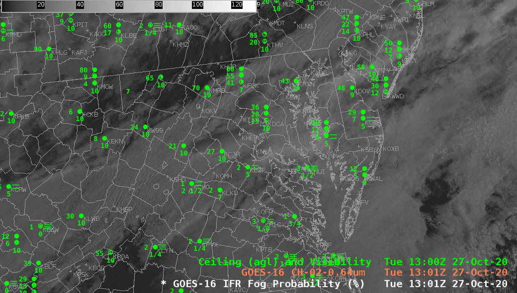
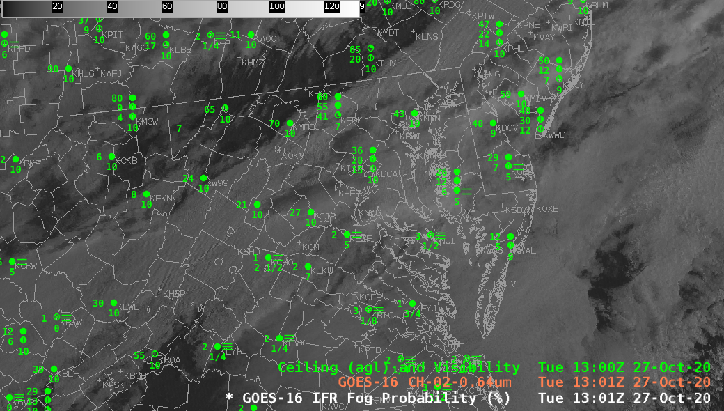
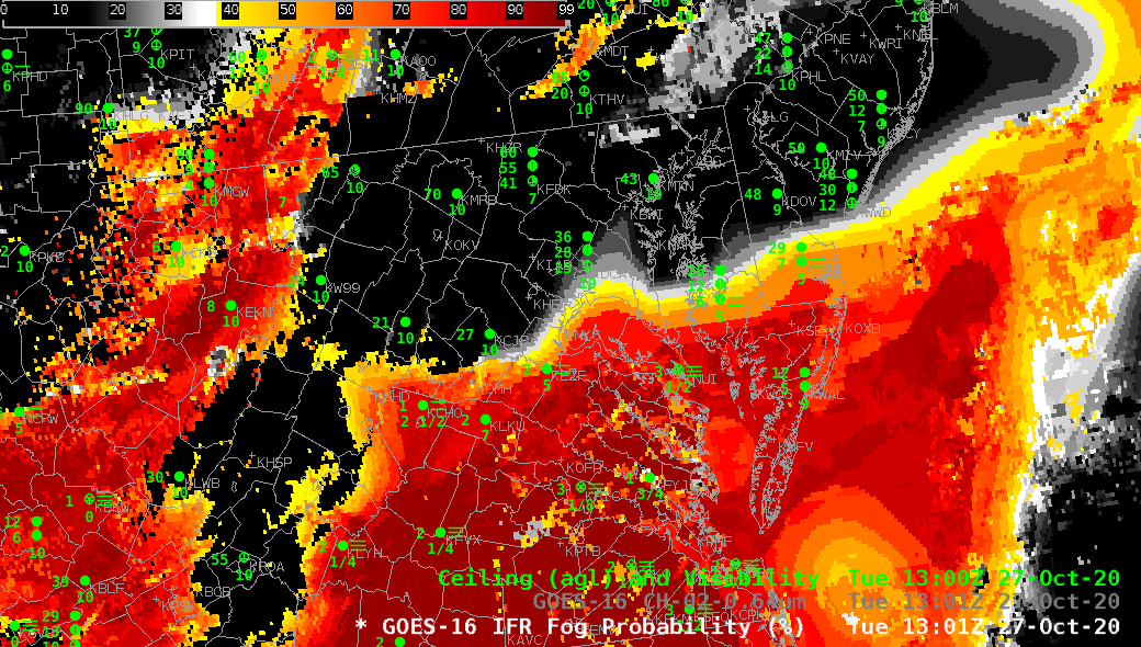
Visible imagery (0.64 µm) toggled with the IFR Probability fields at 1301 UTC, below, show how IFR Probability fields can better discriminate between stratus and fog than visible imagery alone.
GOES-16 Band 2 Visible (0.64 µm) and IFR Probability, 1301 UTC on 27 October 2020 (Click to enlarge)
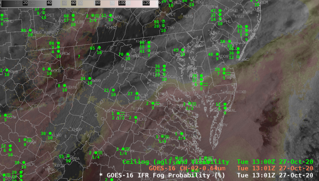
Use IFR Probability fields to identify regions that have low ceilings and reduced visibilities when Visible imagery (in the day) and Night Fog Brightness Temperature difference (at night). During the day time, this can be achieved by displaying both images at once.
GOES-16 IFR Probability underneath the Visible (0.64 µm) imagery, 1301 UTC, 27 October 2020 (with a transparency alpha of 0.9 applied; click to enlarge)
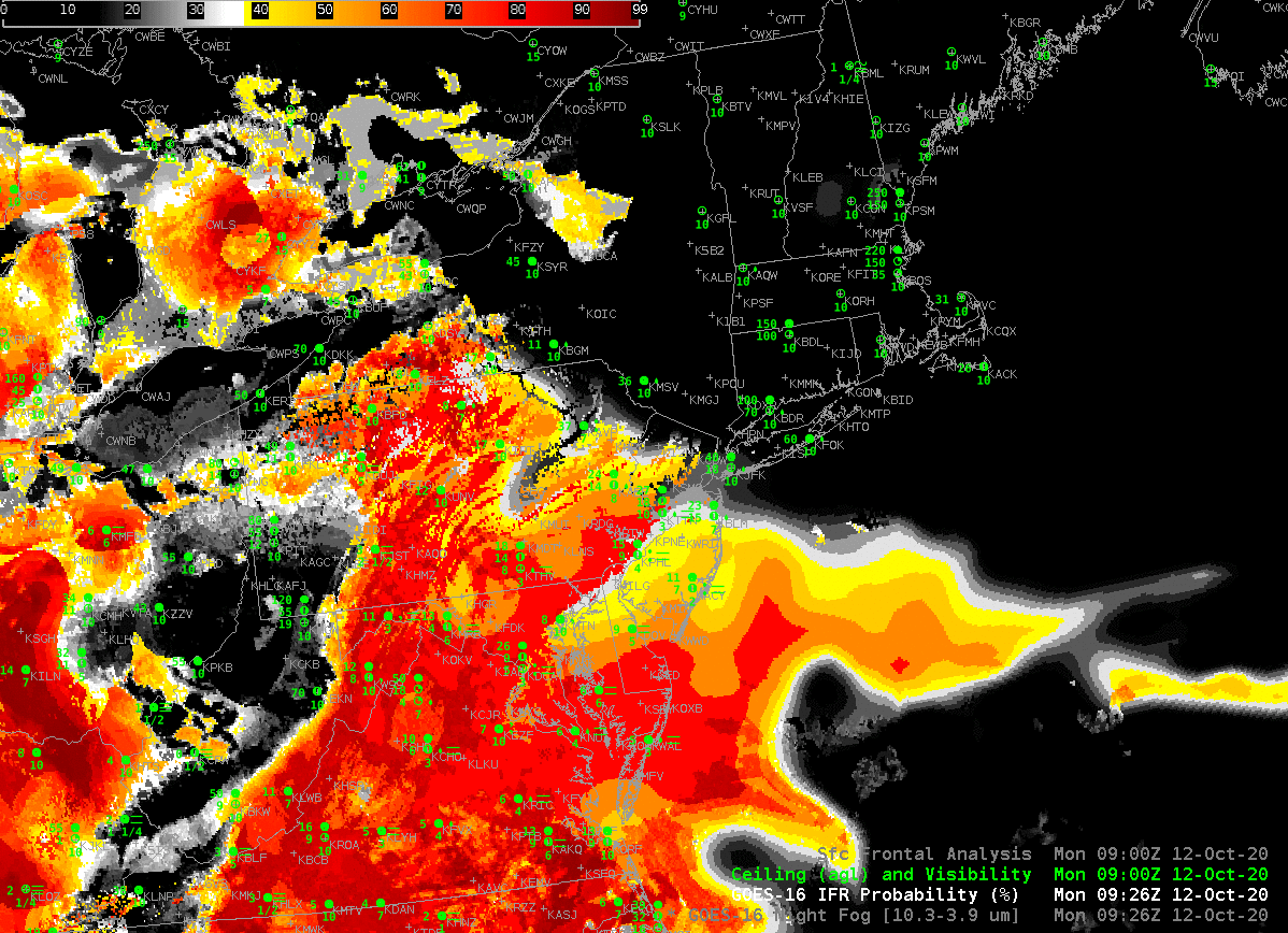
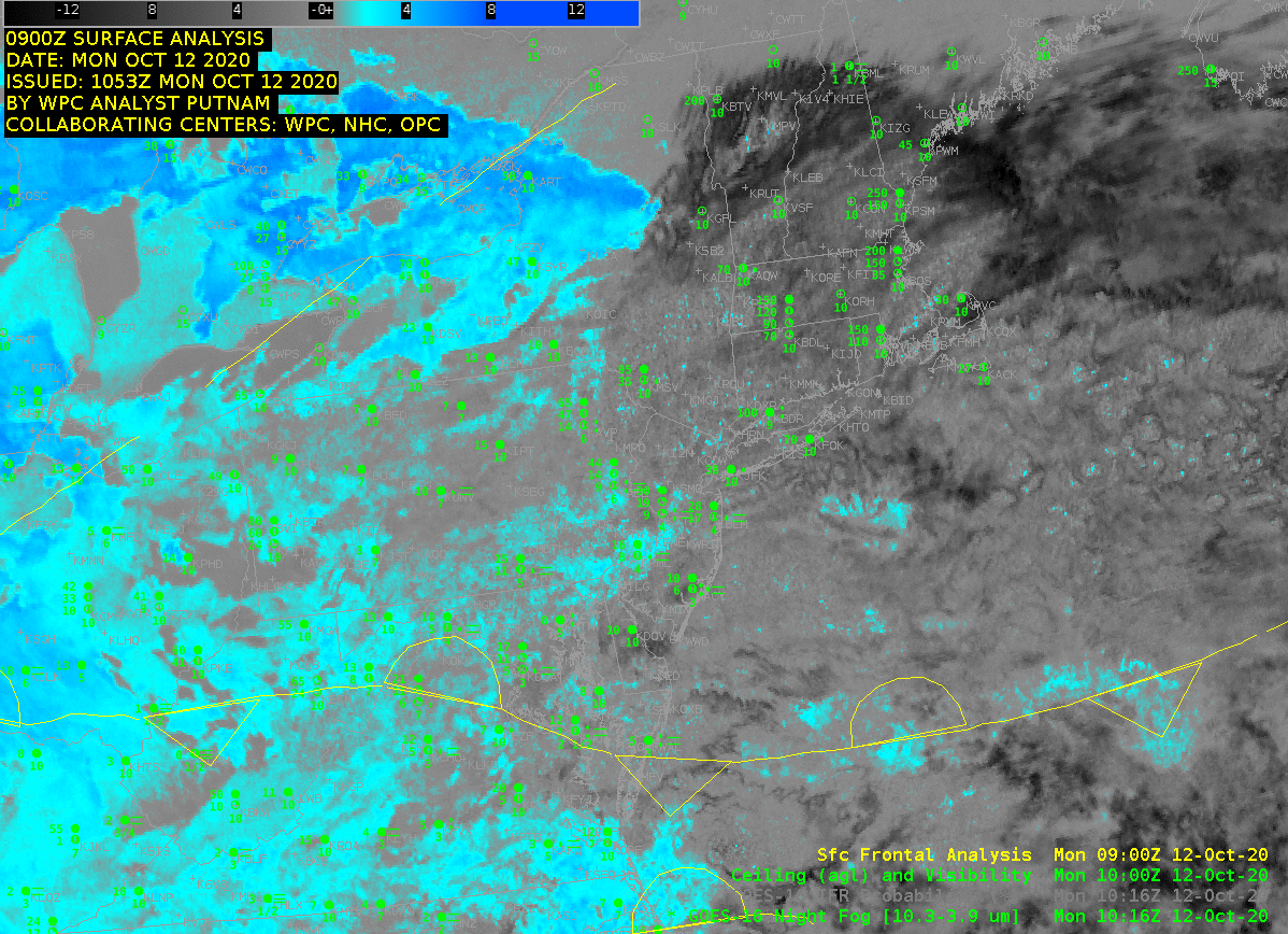
GOES-16 IFR Probability, 0926 – 1101 UTC on 12 October 2020 (Click to enlarge)
The New York City area has 3 major international hubs for which ceiling/visibility observations and prediction are critical to efficient operations. IFR Probability fields use both satellite data and Rapid Refresh model data and can supply information about low-level conditions even where mid-level or upper-level clouds obscure a satellite’s view of low clouds. The example above shows very slow northeastward progress of an area of potential IFR conditions towards New York.
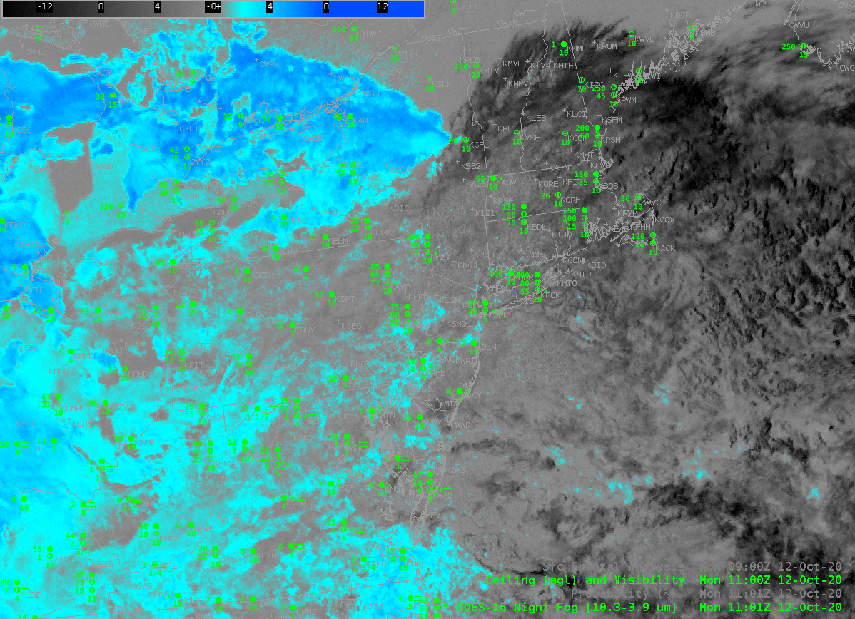
Satellite-only data, below, in the form of the night fog brightness tempreature difference from GOES-16, does not give a useful signal for the low clouds along the east coast. A conclusion: Use IFR Probability to monitor the progress of low clouds when multiple cloud decks are present.
GOES-16 ‘Night Fog’ Brightness Temperature Difference (10.3 µm – 3.9 µm) field, 1006-1101 UTC, 12 October 2020 with 0900 UTC frontal analysis overlain on first image (Click to enlarge)GOES-16 IFR Probability and GOES-16 ‘Night Fog’ Brightness Temperature Difference (10.3 µm – 3.9 µm) field, 1101 UTC, 12 October 2020 (Click to enlarge)
The toggle above, between IFR Probability and the Brightness Temperature Difference demonstrates and underscores (1) how IFR Probability can fill in regions under low clouds (in Delmarva and New Jersey, for example), and screen out regions with mid-level stratus (over eastern Lake Ontario the surrounding land, and over eastern Ohio, for example).
IFR Probability fields are supplied to AWIPS (TOWR-S Build 19) via the SBN.
Fog developed over North and South Carolina (some of this region has been cloudy and wet for much of the past week; here is a weekly precipitation total from this site) on the morning of 19 June 2020; the screenshot above, from this site, shows a sigmet related to the IFR conditions present:
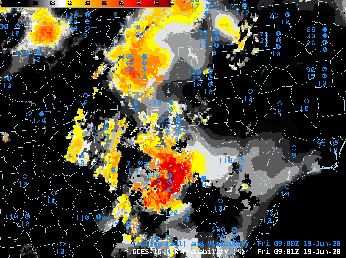
How did GOES-R IFR Probability capture this event? The animation below, from 0900 to 1306 UTC, shows generally high IFR Probabilities over most of the region. There are stations where IFR conditions are occurring and IFR Probabilities are low: the Columbus County Municipal Airport (KCPC, in southeast North Carolina), for example, shows obstructed ceilings and reduced visibility. This might be a localized sub-pixel scale fog related to the small streams near the airport there. A similarly small-scale fog event may be happening at Macon County airport (K1A5) in western North Carolina. The 0901 UTC Brightness Temperature Difference field shows a signal consistent with valley fog along the Little Tennessee River (see image at bottom)
Note how the signal shows little discernible impact from the rising of the Sun. A strength of this product is that uniformity — in contrast to the Night Fog Brightness Temperature difference field.
GOES-16 IFR Probabilities, 0901 UTC – 1306 UTC on 19 June 2020. Surface observations of ceilings and visibilities shown in blue (Click to enlarge)
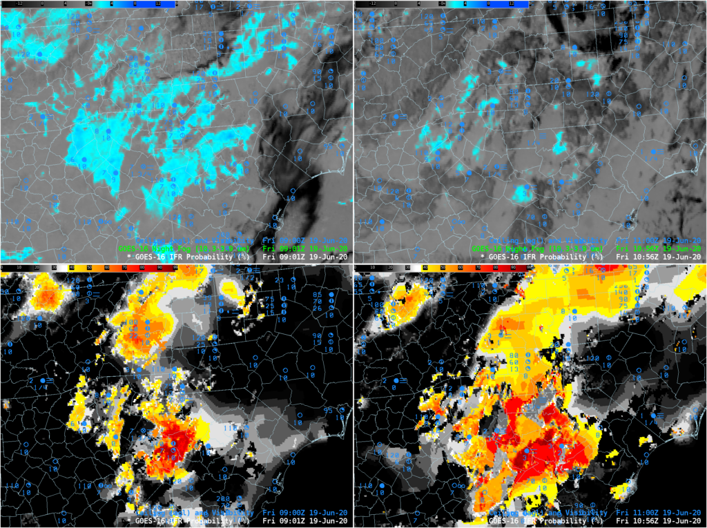
The 4-panel image below shows the ‘Night Fog’ Brightness Temperature Difference (10.3 µm – 3.9 µm, top) at 0901 and 1056 UTC and the IFR Probability fields, also at 0901 and 1056 UTC. IFR probability shows an expansion in the region of low ceilings reduced visibilities, as might be expected to occur around sunrise. The Night Fog Difference field shows a decrease in signal related to the increasing amount of reflected 3.9 µm solar insolation.
Night Fog Brightness Temperature Difference (10.3 µm – 3.9 µm), top and GOES-R IFR Probability, bottom, both at 0901 UTC (let) and 1056 UTC (right) on 19 June 2020.
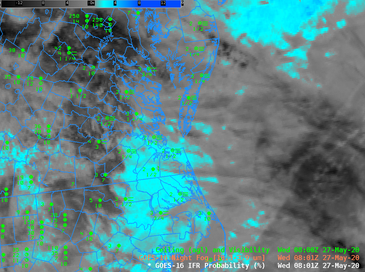
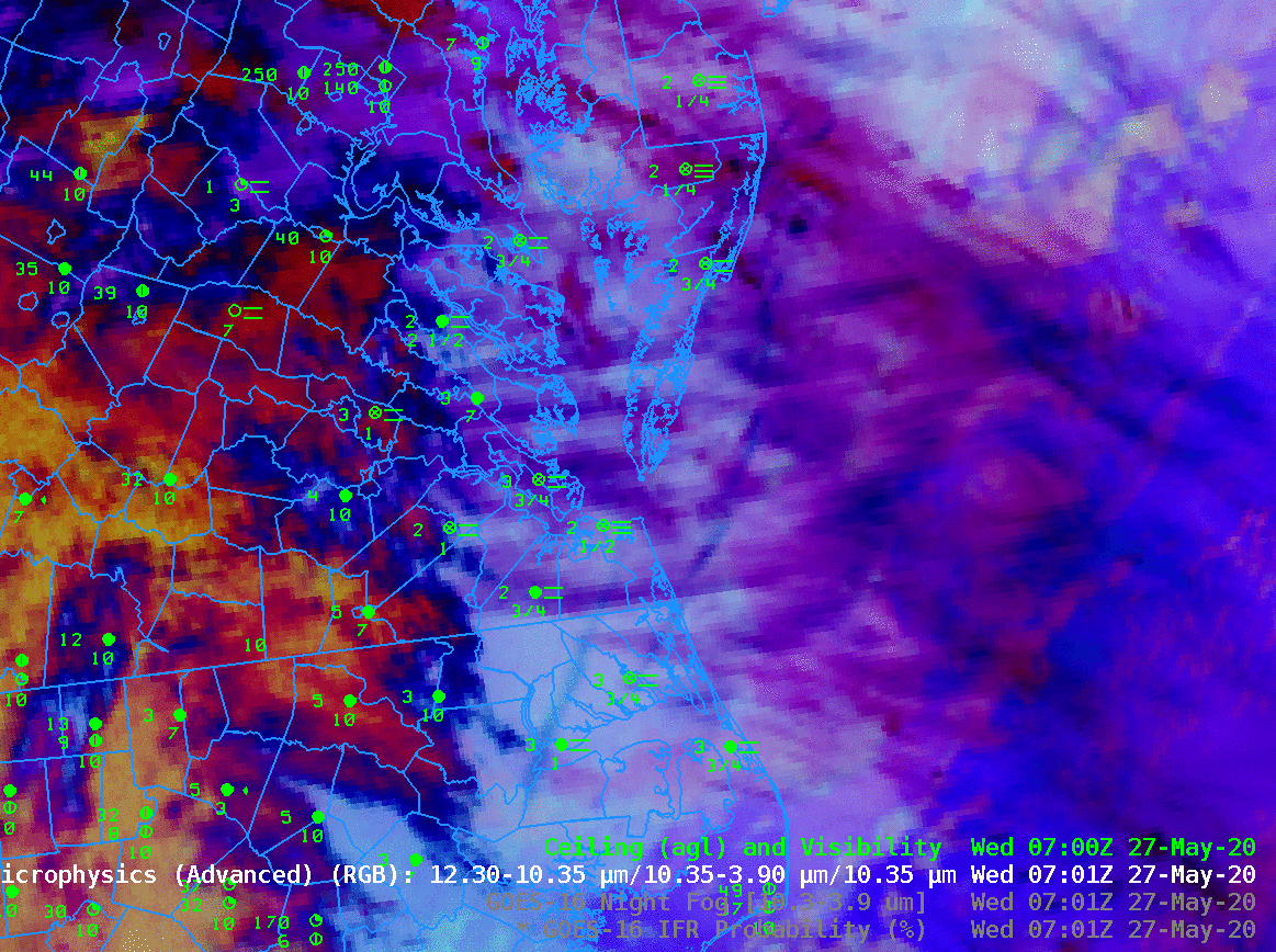
GOES-16 Night Fog Brightness temperature Difference (10.3 µm – 3.9 µm), Night time Microphysics RGB and IFR Probability fields, 0801 UTC on 27 May 2020. Plots of ceilings and visibilities are included (click to enlarge)
Dense Fog was widespread over southeast Virginia on 27 May 2020. The toggle above compares the Night Fog Brightness Temperature Difference field, Night Time Microphysics RGB, and GOES-R IFR Probabilities computed with GOES-16 data and Rapid Refresh Model output, all at 0801 UTC. A challenge with satellite-only detection of low ceilings/poor visibility is that high clouds get in the way. For example, consider the satellite-only signal at Richmond, with 1/4-mile visibility and 200-foot ceilings. Low clouds are not easily detected in that region by satellite; only the GOES-R IFR Probability field (which blends satellite detection of clouds with model estimates of low-level saturation) correctly suggests the transportation hazard that is present there (and extending some distance to the north and west!)
GOES-16 Night Fog Brightness Temperature Difference (10.3 µm – 3.9 µm) field, 0701-1326 UTC on 27 May 2020 (Click to enlarge)
The animation of the night Fog brightness temperature difference field, above, the ‘green’ component of the night time microphysics RGB, shown below, shows a second challenge of using this product for fog detection: the signal is lost (or, at best, changes) as the Sun rises. The RGB product shows the same challenges in fog/low stratus detection that are present in the channel difference field above: high clouds mask the signal, and the signal changes as the sun rises. (Contrails show up very nicely in both however.)
GOES-16 Night Fog Microphysics RGB, 0701 – 1326 UTC on 27 May 2020 (Click to enlarge)
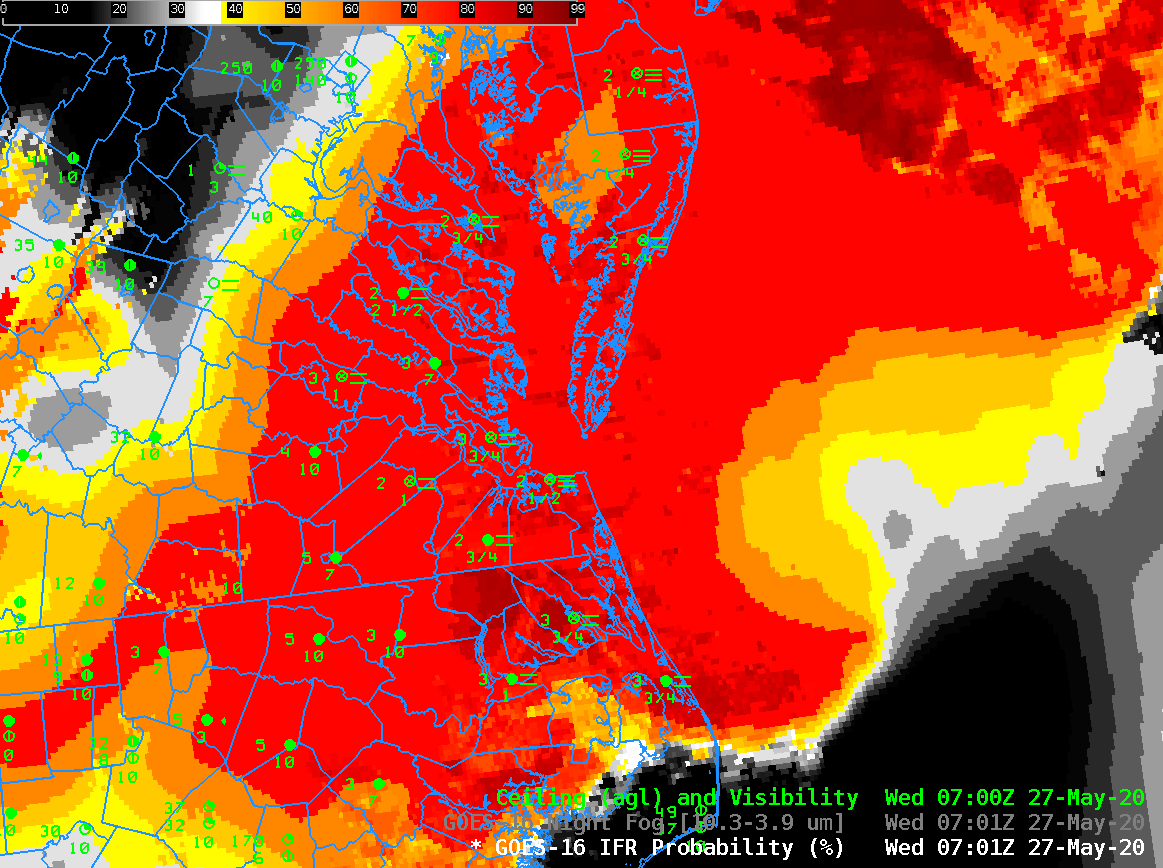
GOES-R IFR Probability fields, below, do a much better job characterizing the horizontal extent of the low clouds early in the animation, and in highlighting the region where visibility reductions persist through sunrise, namely from Hampton Roads northeastward along the coast.
GOES-16 IFR Probability fields, 0701-1326 UTC on 27 May 2020 (Click to enlarge)
GOES-16 ABI Band 2 (0.64 µm) Visible Imagery, 1000-1700 UTC on 11 May 2020
Frontal passage with extratropical cyclones will frequently be accompanied by low ceilings and reduced visibilities, that is, IFR conditions. A loop of visible imagery, above, suggests a surface cyclone (surface analyses are shown below) but it is difficult to determine from the imagery where low ceilings and reduced visibilities are present. Continue reading →
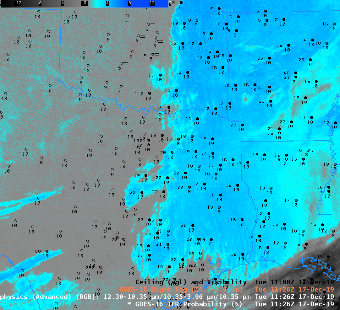
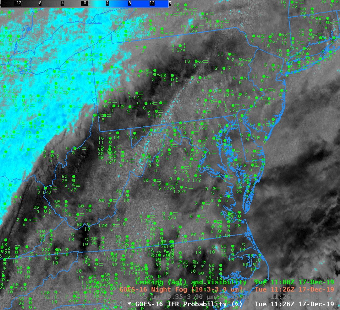
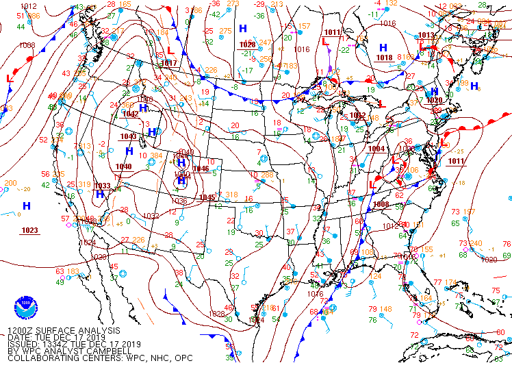
GOES-16 Brightness Temperature Difference (10.3 µm – 3.9 µm), Nighttime Microphysics RGB and IFR Probability Fields, 1126 UTC on 17 December 2019. Also included are sky conditions, ceilings and visibilities in black or green.
Fog and low clouds were widespread over the eastern half of the United States on 17 December 2019. In this example over ArklLaTex the Brightness Temperature Difference suggests low stratus clouds over the region, and the Nighttime Microphysics shows a signal congruent with low clouds. Note, however, that observations over much of the region do not suggest IFR conditions are present. Accordingly, IFR Probability shows fairly low probabilities in this region, with values increasing to the north where visibilities decrease. IFR Probability fields screen out regions of elevated stratus because the Rapid Refresh model in this region does not suggest low-level saturation. Over northeast Oklahoma and northwest Arkansas, however, saturation at low levels is more likely and IFR Probabilities there are larger.
GOES-16 Brightness Temperature Difference (10.3 µm – 3.9 µm), Nighttime Microphysics RGB and IFR Probability Fields, 1126 UTC on 17 December 2019. Also included are sky conditions, ceilings and visibilities in green.
At the same time, high clouds overspread most of the east coast as a storm moved through the area. The high clouds prevent the satellite from seeing low clouds, so both the Brightness Temperature Difference and the Nighttime Microphysics RGB will not have a signal that comports with low stratus detection. However, IFR Probability includes a signal from the Rapid Refresh model if that model shows low-layer saturation in a region of multiple cloud layers; IFR Probability has a strong signal on this date over the east coast were clouds and fog are widespread. IFR Probability also shows IFR Conditions under the low clouds that the satellite does detect over eastern Ohio, and correctly notes the a region of higher ceilings over West Virginia, western Virginia and eastern Tennessee.
GOES-16 Brightness Temperature Difference (10.3 µm – 3.9 µm), Nighttime Microphysics RGB and IFR Probability Fields, 1126 UTC on 17 December 2019. Also included are sky conditions, ceilings and visibilities in green.
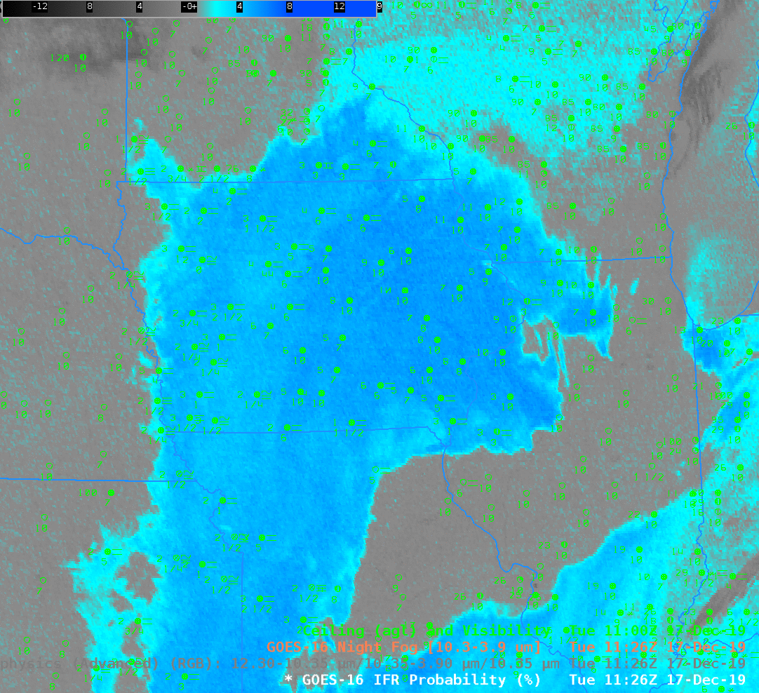
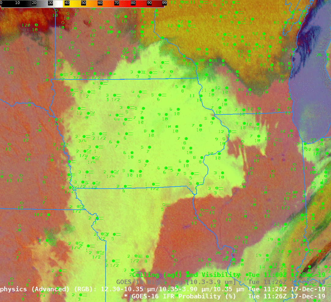
When high clouds are not present, there are different equally good ways to estimate low clouds, and that’s shown above. The Brightness Temperature Difference fields, the Nighttime RGB and the IFR Probability fields all tell a similar tale: Much of Iowa and regions to the south and northeast have low ceilings and reduced visibility.
Careful observers to the toggle note that the RGB has a different color over Wisconsin compared to Iowa. In part this is because the Brightness Temperature Field has values that are smaller over Wisconsin. A bigger driver of the color difference, however, is the 10.3 µm brightness temperature — the blue component of the Nighttime Microphysics RGB. Values are around -25º C over Wisconsin, and closer to -10º C over Iowa!
Nighttime Microphysics RGB and Band 13 10.3 µm Brightness Temperature, 17 December 2019
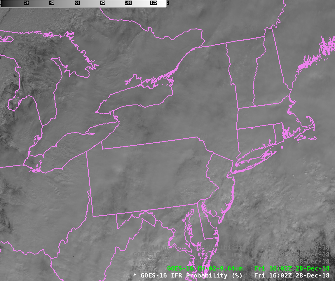
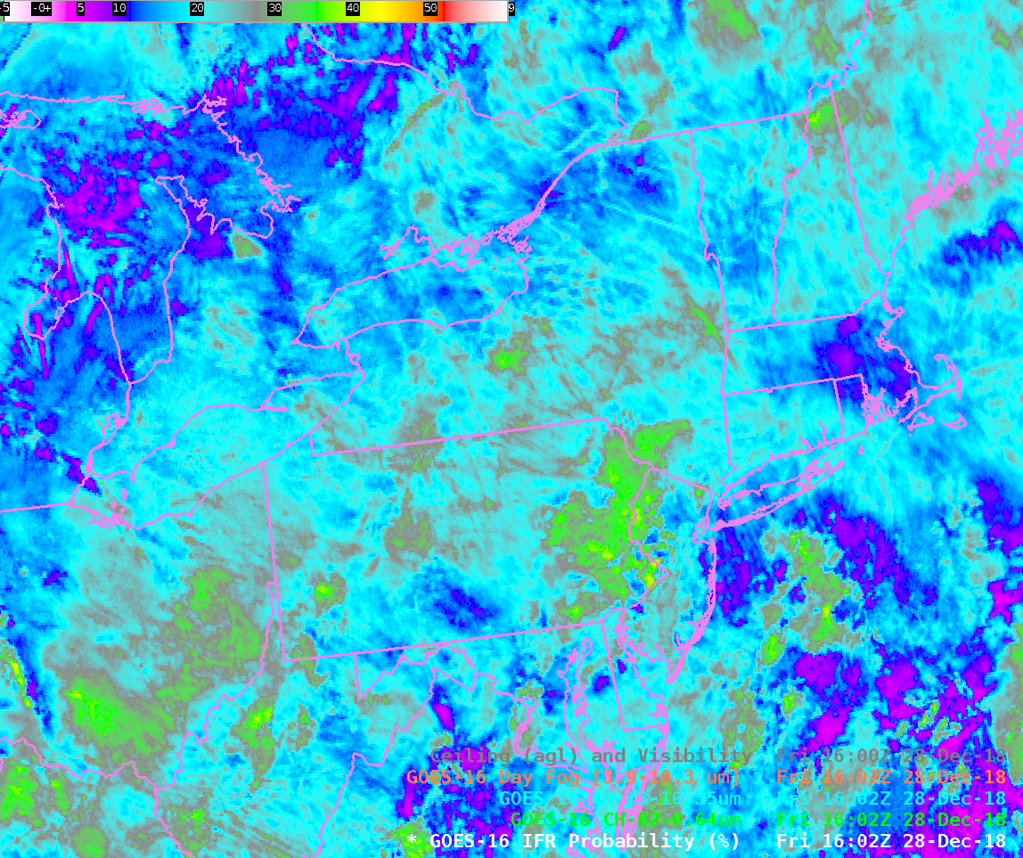
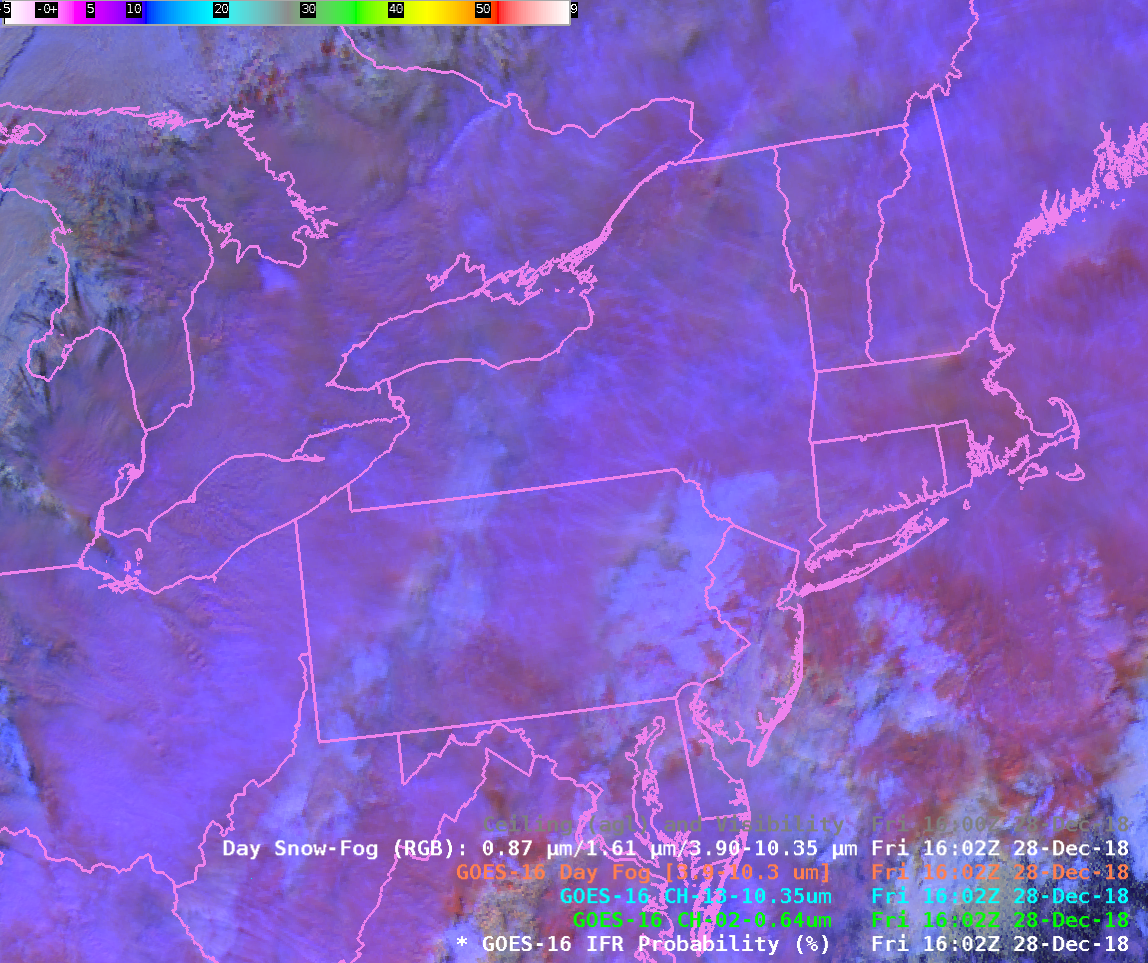
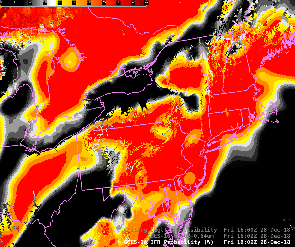
GOES-16 ABI Band 02 (0.64 µm), Band 13 (10.3 µm), Day Fog Brightness Temperature (3.9 µm – 10.3 µm), Day Snow Fog RGB and Band 5 (1.61 µm) at 1602 UTC on 28 December 2018 (Click to enlarge)
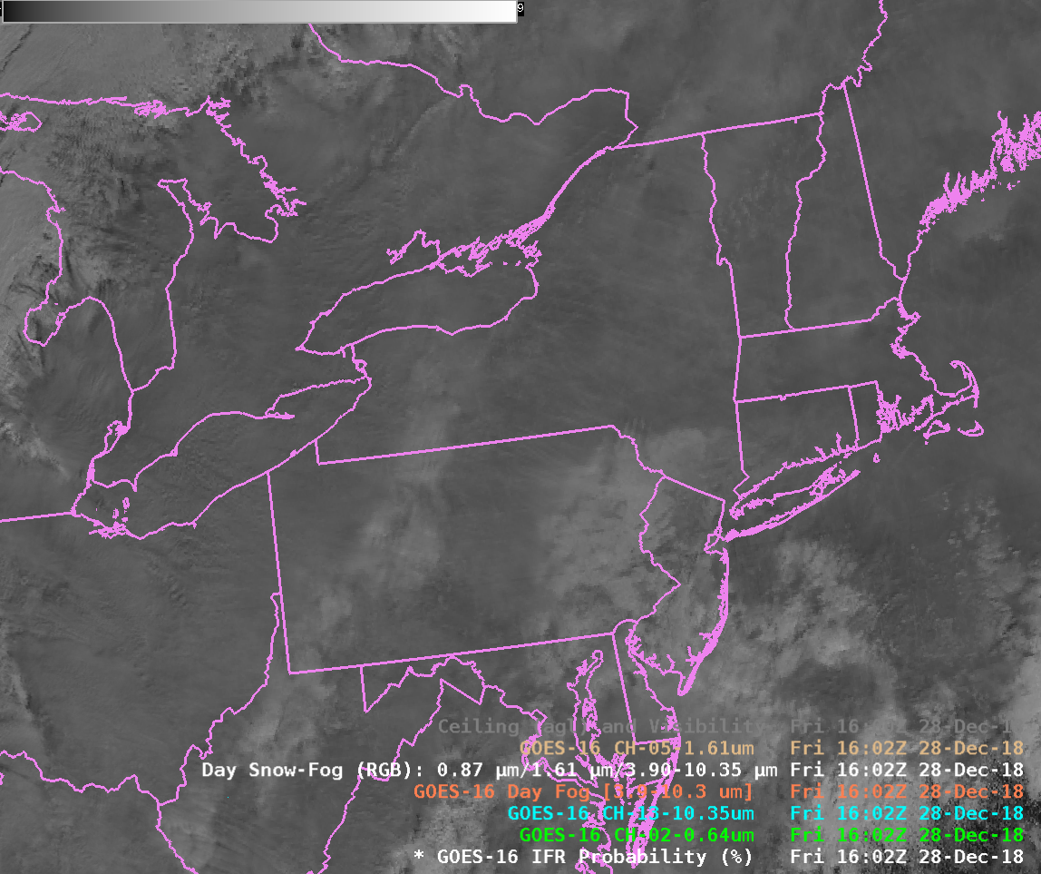
Consider the toggle of visible imagery below, with and without surface observations of ceilings and visibility. It is a difficult prospect to relate the top-of-cloud reflectance (which is what the visible imagery gives you!) to the ceilings beneath the cloud.
GOES-16 ABI Band 02 (0.64 µm) with an without surface observations of ceilings and visibility at 1602 UTC on 28 December 2018 (Click to enlarge)
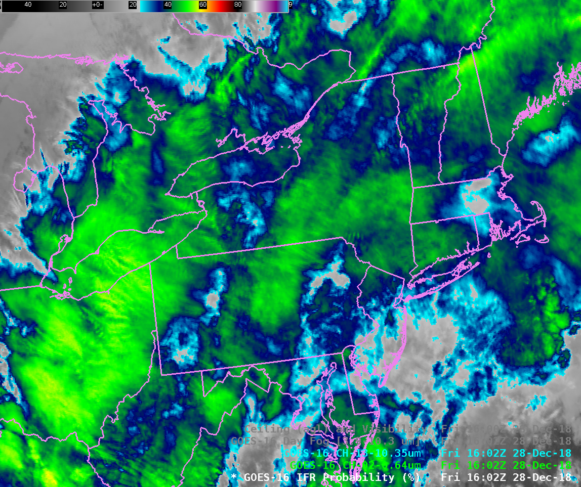
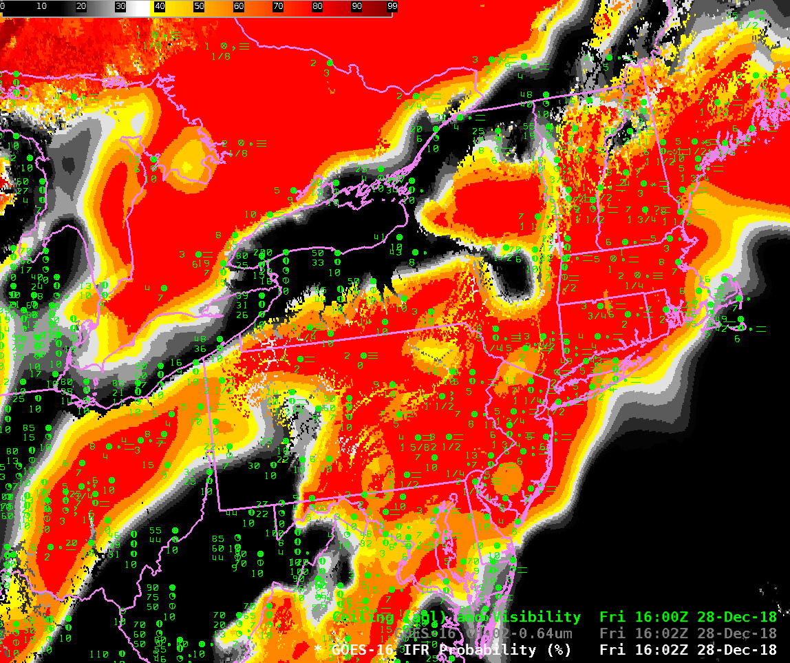
GOES-16 IFR Probability fields blend satellite observations of cloud with Rapid Refresh model data that predicts saturation near the surface. That model data, incorporated into a statistical prediction of IFR conditions, allows the field to outline the regions where low ceilings and reduced visibilities occur, as shown in the toggle below with and without observations. (Click here to see the Visible and IFR Probability fields toggled). The inclusion of near-surface saturation values extracted from the Rapid Refresh model allows the IFR Probability field to discriminate between low ceilings/fog — as over central Pennsylvania, Massachusetts and central Ohio (among other places) — and mid-level stratus — as over southwestern Pennsyvlania and surrounding Lakes Erie and Ontario (among other places).
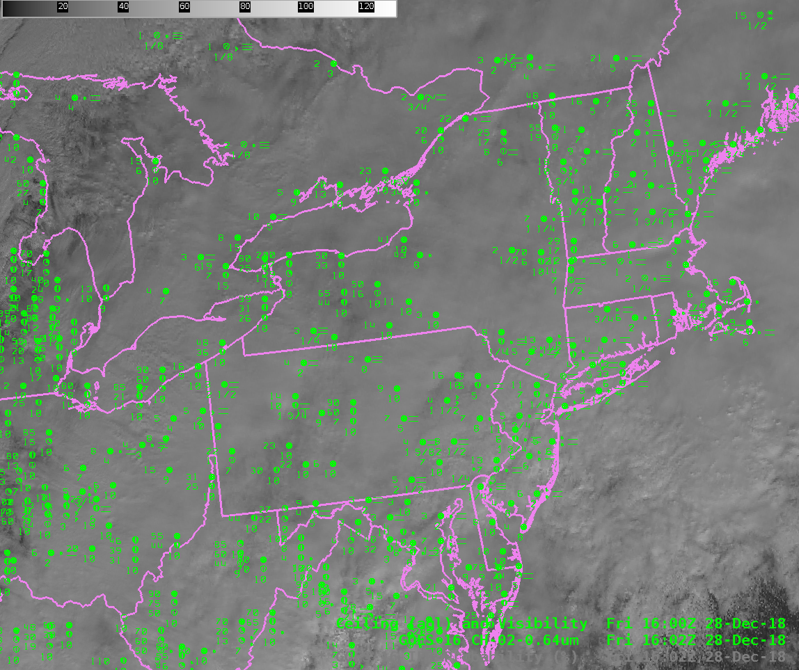
GOES-16 IFR Probability with surface observations of ceilings/visibilities at 1602 UTC on 28 December 2018 (Click to enlarge)
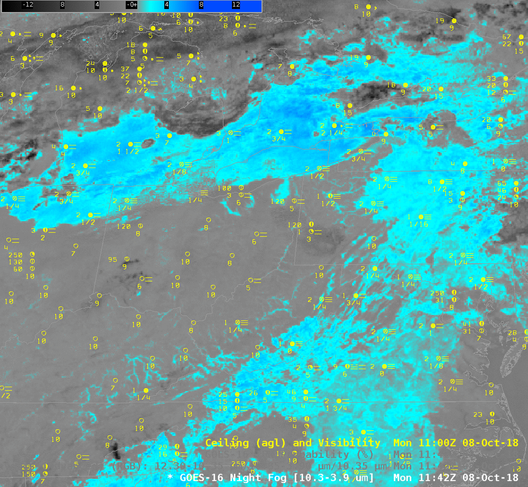
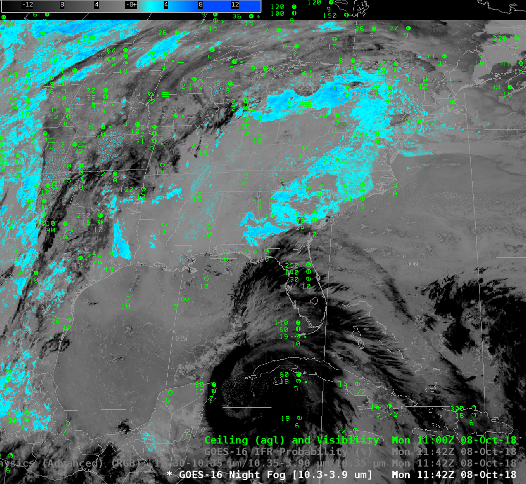
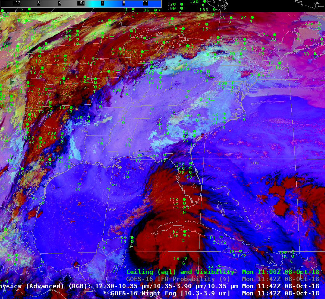
GOES-16 Night Fog Brightness Temperature Difference (10.3 µm – 3.9 µm), Advanced Night Time Microphysics RGB, and GOES-16 IFR Probability fieds at 1142 UTC on 8 October 2018 (Click to enlarge)
Fog and low stratus were widespread on 8 October over the Plains, in particular over Iowa and Minnesota. What satellite tools exist to highlight such regions of lowered ceilings and reduced visibility?
When IFR conditions — fog and low stratus — occur with extratropical cyclones that generate multiple cloud layers, satellite detection of low clouds is difficult because higher clouds get in the way of the near-surface view. The animation above steps through the Night Fog Brightness Temperature Difference (10.3 µm – 3.9 µm; low clouds in the default enhancement are cyan), the Nighttime Microphysics Red-Green_blue (RGB) composite (low clouds in the RGB are cyan to yellow, depending on the temperature) and the GOES-R IFR Probability field (Probabilities for IFR conditions are highest in orange/red regions) for 1142 UTC on 8 October 2018, when low ceilings were widespread over the Plains and East Coast. Abundant high clouds rendered the Night Fog Brightness Temperature difference product (and, by extenstion, the Night Time Microphysics RGB, because the RGB uses the Night Fog Brightness Temperature Difference as its ‘Green’ Component) ineffective in outlining potential regions of low clouds. In contrast, the IFR Probability field was able to highlight low clouds under the high clouds because it fuses satellite data (ineffective at this time) with Rapid Refresh model estimates of low-level saturation.
There are regions — southern Lake Erie, for example — where the lack of high clouds allows the Brightness Temperature Difference field, and the Nighttime Microphysics RGB to operate with success in identifying low clouds.
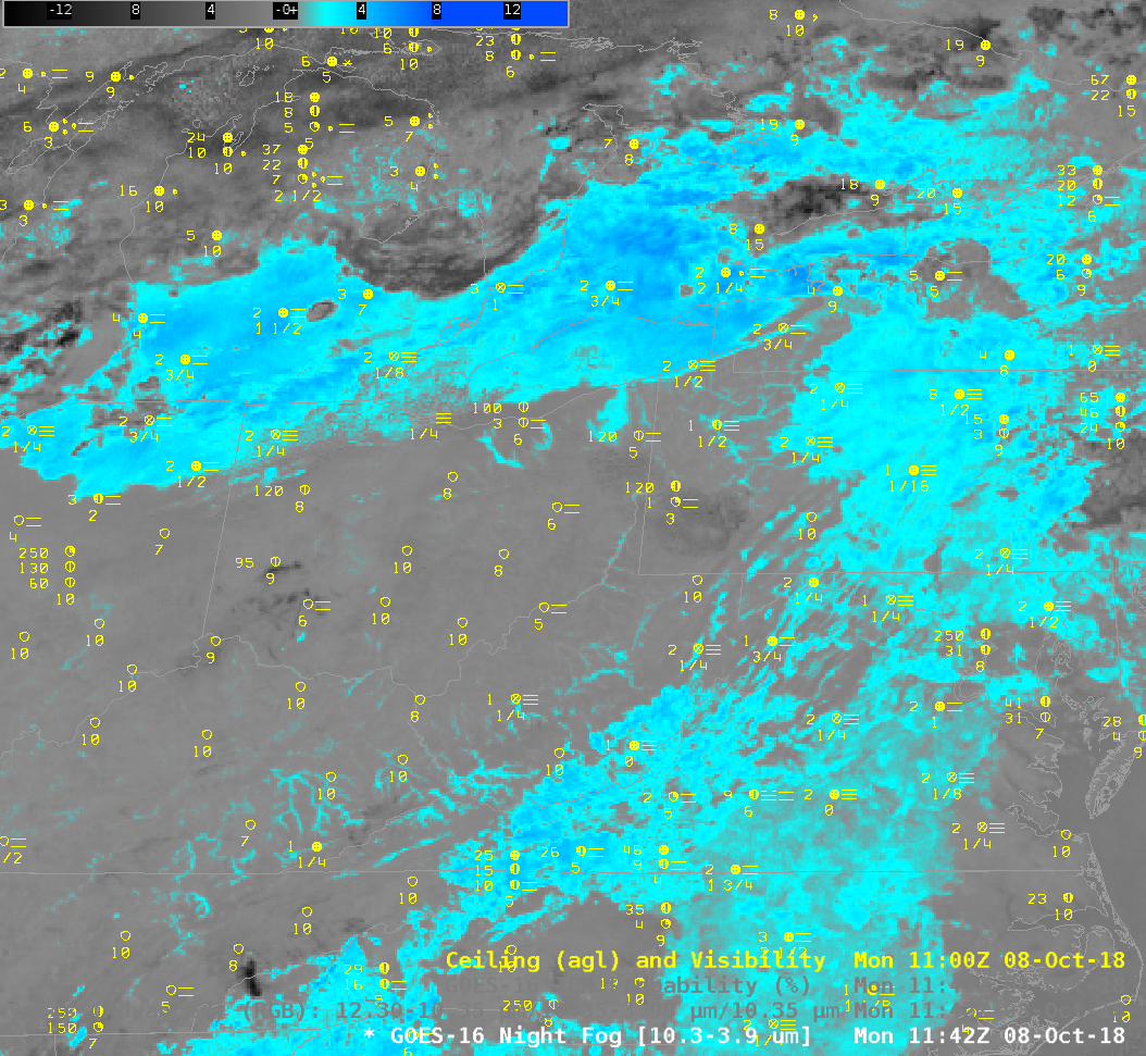
The toggle below shows the Night Fog Brightness Temperature Difference and the IFR Probabiity fields over the eastern portion of the country. Very small-scale (in the horizontal) features, such as river fog, are a challenge for IFR probability because the Rapid Refresh horizontal resolution of 13 km may not resolve river valleys.
GOES-16 Night Fog Brightness Temperature Difference (10.3 µm – 3.9 µm) and GOES-16 IFR Probability fieds at 1142 UTC on 8 October 2018 (Click to enlarge)
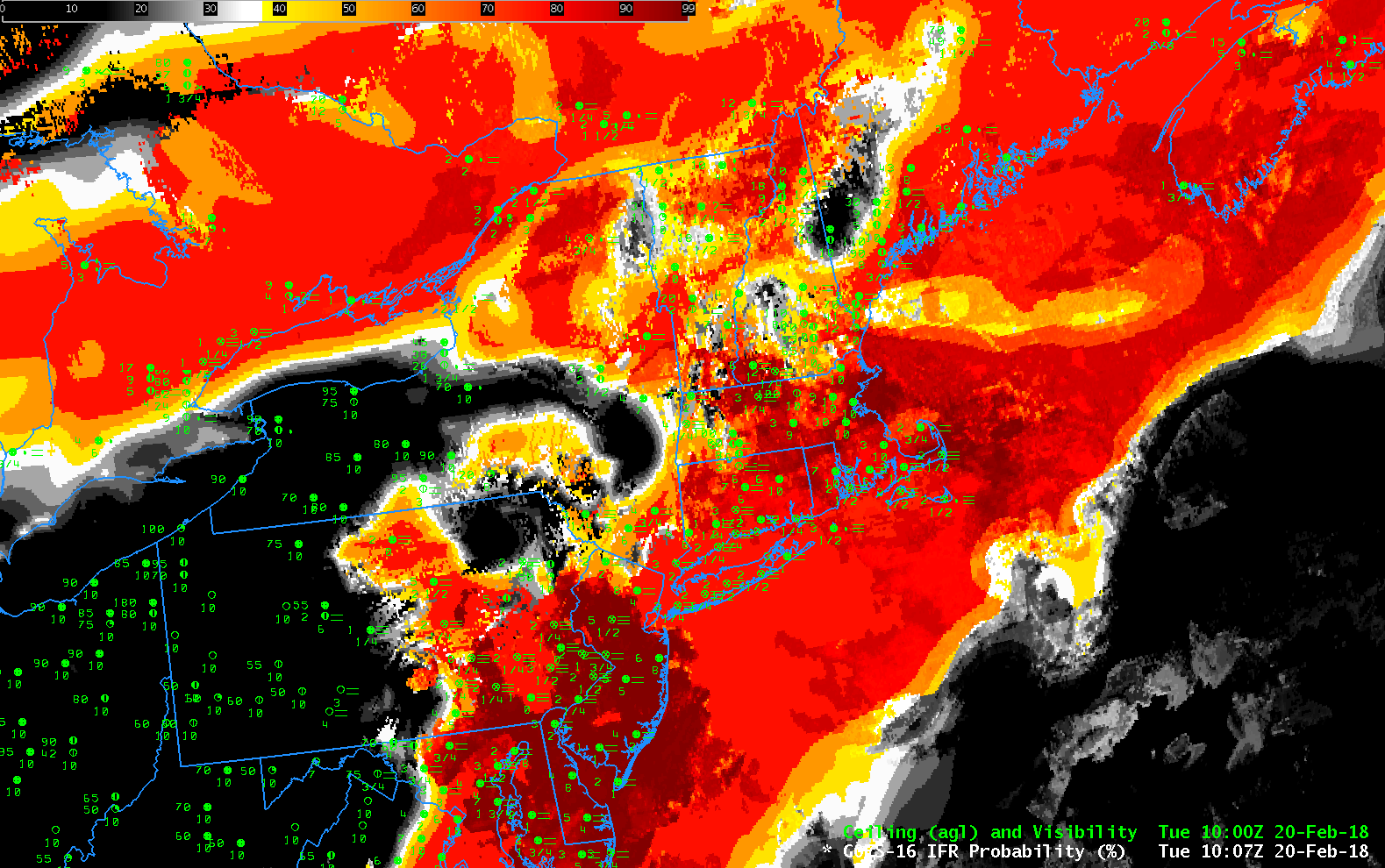
GOES-16 IFR Probability, 1007 UTC on 20 February 2018, along with surface observations of ceilings and visibilities (Click to enlarge)
A complex set of Low Pressure systems over the eastern half of the United States brought multiple cloud layers and IFR conditions to the northeastern United States on 20 February. The image above shows the IFR Probability field at 1007 UTC. IFR Conditions are apparent from the Chesapeake Bay northeastward through southeastern Pennsylvania and New York and coastal New England, as well as over southeastern Ontario Province in Canada and the Canadian Maritimes. These are also regions where IFR Probabilities are high, generally exceeding 80%. In regions where IFR conditions are not observed (Western Pennsylvania and Ohio, for example), IFR Probabilities are generally small.
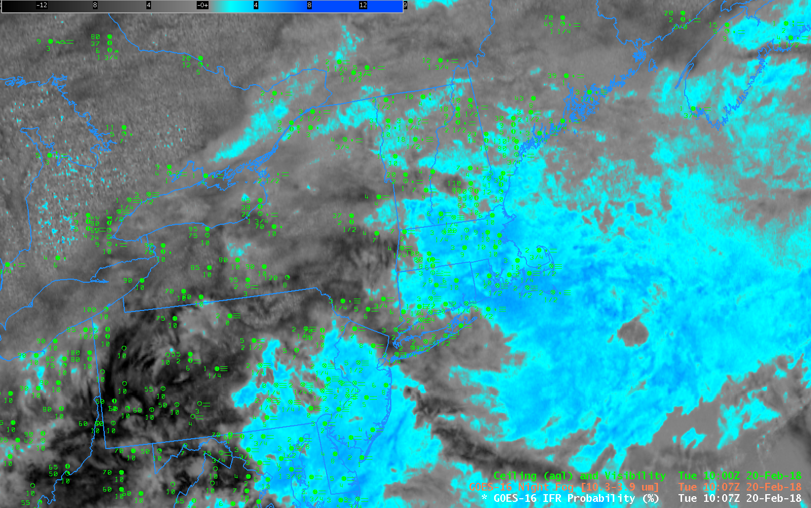
When multiple cloud decks are present, as occurred on 20 February, satellite-only detection of low clouds is a challenge, as shown with by the brightness temperature difference field (10.3 µm – 3.9 µm), called the ‘Night Fog’ difference in AWIPS, below. High and mid-level clouds (grey/black in the enhancement used) make satellite detection of low-level stratus impossible. So, for example, stations with IFR conditions over Long Island sit under a much different enhancement in the brightness temperature difference field compared to stations with IFR conditions over southern New Jersey and southeastern Pennsylvania.
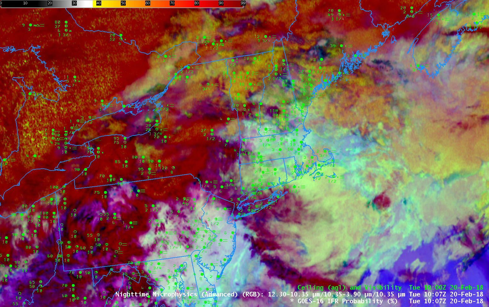
Because the Brightness Temperature Field cannot view the low clouds, the Nighttime Microphysics RGB (shown below the Brightness Temperature Difference field) similarly cannot identify all regions of low, warm clouds — typically yellow or cyan in that RGB.
Night Fog Brightness Temperature Difference field (10.3 µm – 3.9 µm) at 1007 UTC on 20 February 2018, along with surface observations of ceilings and visibilities (Click to enlarge)
NightTime Microphysics RGB at 1007 UTC on 20 February 2018, along with surface observations of ceilings and visibilities (Click to enlarge)


