Monthly Archives: August 2012

Emissivity properties in a drought

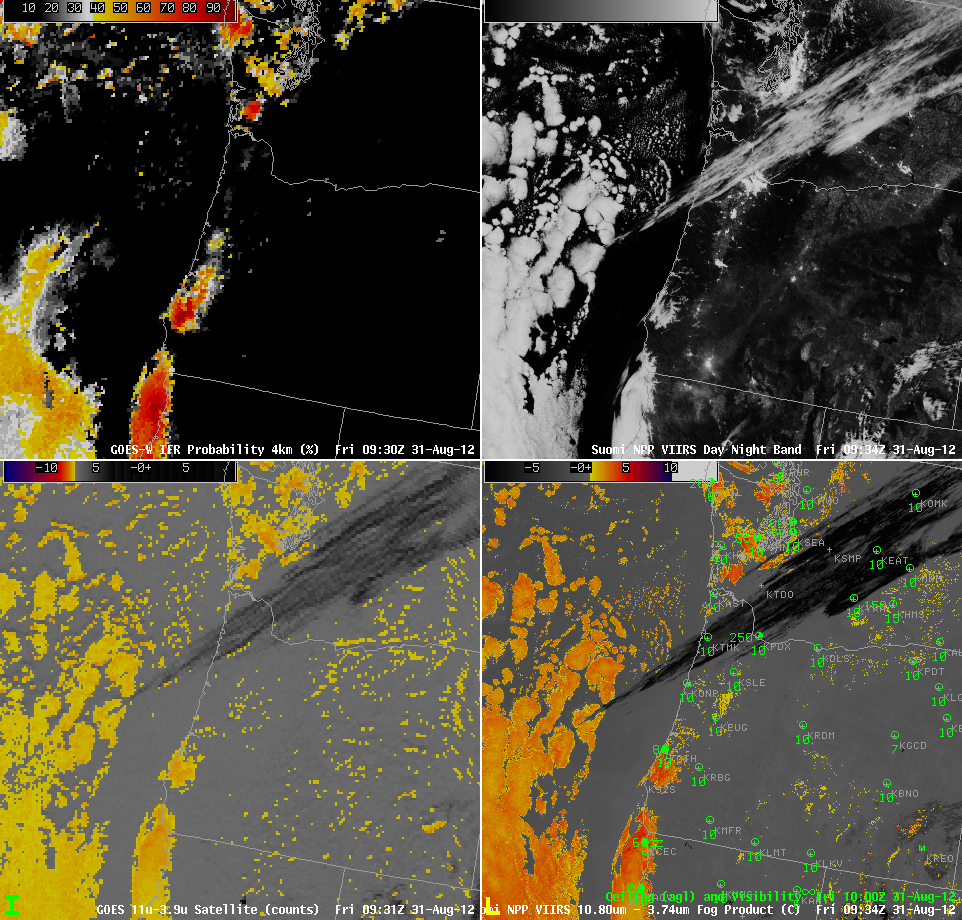
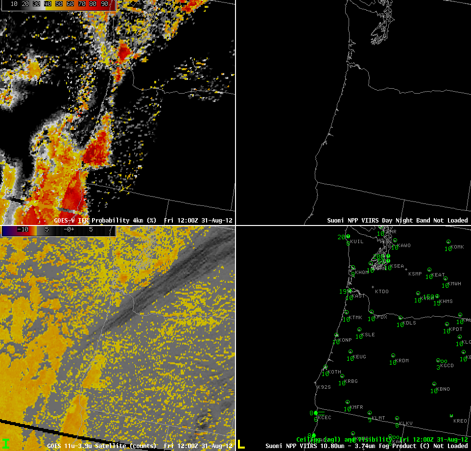
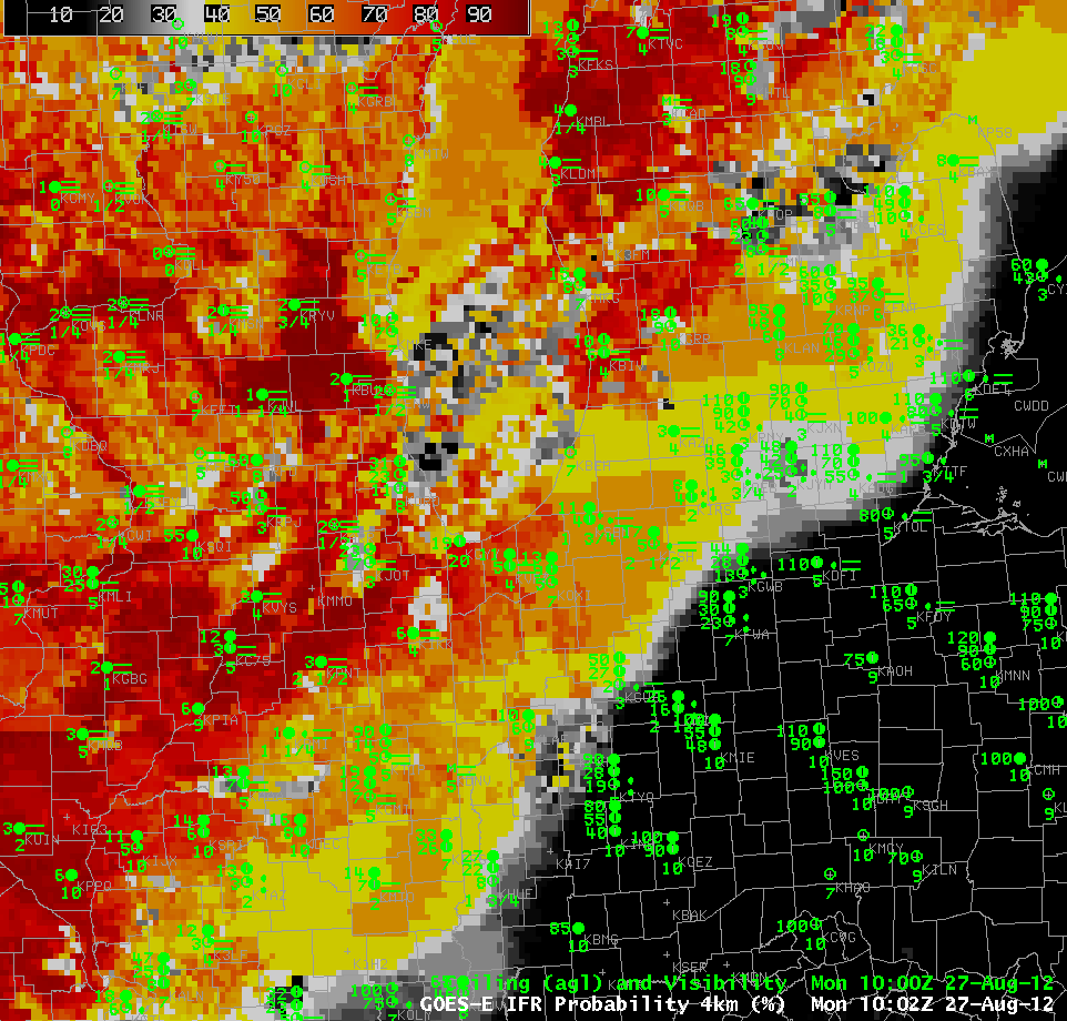
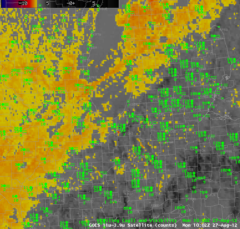
GOES-R IFR Probabilities (upper left), Total Precipitable Water (the so-called ‘Blended Product’) (upper right), 10.7 µm – 3.9 µm Brightness Temperature Difference (lower left), Enhanced Water vapor imagery with surface observations (lower right)

The driving mechanism in the brightness temperature difference product, the heritage method for detecting fog and stratus from satellites, keys on differences in the emissivity of water clouds at 3.9 µm versus the emissivity at 10.7 µm.  Water clouds do not emit 3.9 µm radiation as a blackbody does, but they do emit 10.7 µm radiation almost as a blackbody.

As ground dries out in a drought, its emissivity changes. Those changes are a function of wavelength.  This example is from early morning on 31 August, as the remnants of Isaac slowly spread northward.  The brightness temperature difference shows a strong signal around the cirrus canopy of the storm.  These highlighted regions arcing from Kansas to Illinois have suffered extreme drought all summer.  The satellite signal is so strong in this case over the very dry Earth — because of the changed emissivity properties of the parched Earth — that it cannot be overcome by the model parameters that are used.  As a result, IFR probabilities are high over Indiana and Illinois where no IFR conditions are observed.

GOES-R Fog and the Day/Night Band on VIIRS

GOES-R IFR Probabilities (upper left), Suomi/NPP VIIRS Day/Night Band (upper right), Brightness temperature difference (10.7 micrometers – 3.9 micrometers) from GOES (lower left), Brightness temrperature difference (11.35 micrometers – 3.74 micrometers) from Suomi/NPP VIIRS (lower right), all around 0930 UTC on 31 August.

The presence of the Day/Night band on the VIIRS instrument on the Suomi/NPP satellite offers a unique method of validating the presence of fog or stratus at night.  During times near full moon (such as the Blue Moon on 31 August), the Day/Night band can detect low clouds using light reflected from the moon.  The GOES-R IFR probabilities show fog and low/stratus over southwestern Oregon;  a larger region of fog/low stratus stretched from just north of Crescent City, CA (where IFR conditions are reported) southward down the coast.  Note also a small patch over southwestern Washington and coastal northwest Washington (where IFR conditions are reported.  Cirrus clouds that prevent the detection of fog/low stratus from satellite are present stretching northeastward from the ocean off the central Oregon coast into central Washington.  There is a small signal in the GOES-R IFR Probability field underneath this upper cloud feature.

GOES-R IFR probabilties (Upper left), Suomi/NPP VIIRS day/night band (upper right), GOES-West Brightness Temperature Difference between 10.7 and 3.9 micrometer channels (Lower left), Observations (Lower right), all around 1200 UTC, 31 August

AT 1200 UTC, some benefits of the GOES-R IFR probability field are apparent.  The noisy signal over central and eastern Oregon is reduced, and a signal is present also underneath the thin cirrus streak that persists over extreme northwest Oregon.

IFR in Alaska when a Large-Scale weather system is present

Animation of 1400 UTC Water vapor imagery, the 10.7 micron infrared image, the brightness temperature difference (10.7 – 3.9), the GOES-R IFR Probabilities computed from GOES data, the GOES-R IFR Probabilities computed from MODIS data, and the surface observations/ceilings.

The loop above cycles through the 1400 UTC Water vapor imagery, the 10.7 micron infrared image, the brightness temperature difference (10.7 – 3.9), the GOES-R IFR Probabilities computed from GOES data, the GOES-R IFR Probabilities computed from MODIS data, and the surface observations/ceilings.  The complex large-scale weather system over northwest Alaska is means that southerly winds over eastern Alaska are drawing moisture and cloudiness northward from the Gulf of Alaska.  Multiple cloud layers in this moist flow means that the traditional method of fog/low stratus detection (the brightness temperature difference between 10.7 and 3.9 micrometers) will be challenged.  Furthermore, on this particular day, IFR conditions (the observation map is below;  stations with IFR conditions are circled in red) are most frequent underneath the multiple cloud layers in the eastern part of the state, and at high levels, such as in the Brooks Range.

The GOES-R IFR probability field suggests higher possibilities of IFR conditions in regions where IFR conditions are observed:  near Anchorage, on the Aleutian peninsula and in the Brooks Range.

Observations over Alaska at 1500 UTC 31 August.  IFR conditions highlighted by red circles.

IFR over SW Alaska

GOES-R IFR Probabilities (upper left) computed from GOES-West, GOES-R IFR Probabilities computed from MODIS (upper right), Visible Imagery (bottom left), Topography (bottom right)

GOES-R probabilities are a fused product between satellite data and the Rapid Refresh model.  Model data are used only where multiple cloud layers are present and or where a single cirrus cloud level exists.  The character of the IFR probability field looks different when model data only is used.  IFR probabilities are lower when only model data are used.

IFR probabilities are well related to observations at Kodiak, for example.  As the higher probabilities increase from the southwest, ceilings lower, and eventually IFR conditions occur.  The better resolution of the MODIS imagery, below, allows far finer-scale structures to be resolved in the imagery.

GOES-R IFR Probabilities (upper left) computed from GOES-West, GOES-R IFR Probabilities computed from MODIS (upper right), Visible Imagery (bottom left), Topography (bottom right)

Note how the smaller probabilities are downwind of the Aleutians.  Visible imagery — at the end of the animation — distinctly shows the clear region.

IFR Conditions in Isaac

GOES-R IFR Probability Field associated with Tropical Storm Isaac

The multiple cloud layers associated with a tropical system, and the extensive cirrus shield that is spawned by rainbands, makes it very difficult for the traditional brightness temperature difference product to be used to highlight regions of low stratus and fog.  This is when model data are vital in a fused product to highlight regions of aviation hazards, as shown in this loop.  There is a change in probability as the Sun rises that is associated with changes in the weights given to various predictors.  The color table suggests a very abrupt change.  In reality, values increase from 10 to 15 percentage points.

Note how well the IFR probability field matches the regions of IFR and near IFR conditions in the loop above.  This is testament to the accuracy of the model data, and to the relationships developed between model fields and IFR observations.

Fog over North Dakota

GOES-East brightness temperature difference (Upper left), GOES-R FLS Product (Upper Right), Ceiling and visibility observations (Lower left), Visible Imagery (Lower right)

Relatively light winds and high dewpoints promoted the development of isolated fog over the Dakotas on the morning of the 29th.  How did satellite-based and satellite-influenced fog detection algorithms perform?

The Brightness Temperature difference field shows returns suggestive of fog or low stratus in regions over western North Dakota — west of the Missouri River — where IFR conditions are not reported.  The GOES-R FLS product suggests a smaller region of fog and low stratus;  there are high probabilities in regions where IFR conditions occur.  However, there are several examples of IFR conditions that are reported at stations just at the edge of the region of high probabilities:  KMHE at 1115 and 1215 UTC, for example.  The isolated nature of the fog in the visible imagery also is suggetive of a more limited fog event than might have been expected given the Fog/Low stratus probabilities.  Note the abrupt change as daytime predictors replace nighttime predictors.  In this case, it seems as though the daytime predictors better handle the small horizontal scale of the fog event.

The morning sounding from KBIS is characteristic of a fog event in a river valley.

Thermodynamic diagram for KBIS at 1200 UTC on 29 August 2012. Note the saturated layer at the surface.

GOES-R Fog/Low Stratus in Alaska

GOES-R IFR Probabilities from GOES-W (Upper Left) and from MODIS (Upper Right); GOES-W color-enhanced IR Imagery (Bottom Left), Alaska Topography (Bottom Right).  Station Observations including visibilities and ceilings above ground level as indicated.

Alaska poses unique challenges in both Fog/Low stratus detection and in aviation forecasting.  For example, there are very few observation sites — airports — where verification of products can occur.  The abundance of small aircraft — bush aircraft — means that aviation support is critical in remote regions where such aircraft will operate.  Alaska is also far enough north that the GOES-West pixel footprint size is very large, making detection of small-scale fog events difficult.

The series of images above document some of these issues.  The GOES-R IFR Probabilities computed with GOES-West data (upper left) and MODIS data (upper right) show similar patterns.  But the far superior resolution inherent in polar orbiters over Alaska results in far greater detail in the MODIS product.  This is a case with multiple cloud layers over northern Alaska (as evidenced by the 10.7 window channel image, lower left);  the enhanced IFR probabilities along the Brooks Range in northern Alaska are mostly model-driven (the model used in that region is the Rapid Refresh (the boundary between the Rapid Refresh and the GFS is apparent in the upper left image over the Bering Sea and over far northern Alaska).  The model suggests IFR conditions are possible in an elevated stratus cloud that surrounds the Brooks Range.  That is, the terrain is rising up into the clouds.

When relatively low IFR probabilities are more likely to mean fog

GOES-R IFR Probabilities over the Midwest, 1000 UTC on 27 August 2012

An important consideration when interpreting GOES-R IFR probabilities is the data being used to compute the probabilities.  When both model and satellite data are used, higher probabilities can result, as over south central and southeastern Wisconsin in the image above where probabilities exceed 90% in a region of IFR conditions.  The pixelated nature of the field there suggests that satellite data are being incorporated into the probability field.  When only model data are used, as over southern Lower Michigan in the image above, lower probabilities will result; however, IFR probabilities are nevertheless observed (as in Kalamazoo (KAZO), for example).  The blockier nature of the IFR probability field is showing that only model data are being used in that region.  The traditional brightness temperature field for that time is shown below. 

Traditional Brightness Temperature Difference Field over the lower Great Lakes, 1002 UTC 27 August 2012.

Importance of Satellite Data in the GOES-

GOES-R IFR Probabilities over Colorado, Kansas and Nebraska, hourly from 0615 UTC to 1415 UTC on 24 August 2012

The loop above shows the importance of satellite data in the GOES-R Fog product.  Only the Satellite information will have sharp cut-offs that are apparent in this imagery.  (The character of the GOES-R IFR field that is described mostly by model data is apparent in the southeast part of this domain at the beginning of the loop when a convective system is moving eastward out of the domina).  Smoothing in model data typically means that sharp cutoffs will not exist.   Note the visibility in Akron, CO, in the center of the image, agrees very well with the GOES-R IFR field.

Fog over the Texas Panhandle

GOES-R IFR Probabilities, and Surface Visibility/Ceilings, from 0432 UTC through 1432 UTC on 22 August 2012

GOES-R IFR Probabilities showed good spatial correlation with observed IFR conditions early in the morning on 22 August 2012.  The spatial characteristics of the field suggest that model-only predictions of the presence of fog/low stratus occurred in regions over west Texas that were overlain by higher clouds.  The Traditional brightness temperature difference product at 1101 UTC, for example, below, shows the characteristic signal of high clouds over parts of west Texas.  There is also a significant region of returns over north central OK/south central Kansas that is not associated with IFR conditions.  The GOES-R IFR product in that region correctly shows low probabilities.

Brightness Temperature Difference from GOES (10.7 – 3.9) at 1101 UTC 22 August.

The upper-air sounding from Amarillo from 1200 UTC confirms the presence of saturated conditions only in the boundary layer.

Skew-T/Ln P Thermodynamic diagram frmo 1200 UTC 22 August 2012 at Amarillo TX