When IFR Probability Fields are stationary

GOES-R IFR Probability Fields computed from GOES-13 on 17 February 2015, times as indicated (Click to enlarge)

Different kinds of fields are used in the computation of IFR Probability fields: fields that can change quickly with time (Satellite observations of brightness temperature difference, satellite observations of cloud type, model output showing low-level moisture); fields that can change slowly with time (Sea surface temperature and surface emissivity fields), and fields that don’t change (Topography). An IFR Probability field that is relatively constant with time, then, as over northern Alabama in the animation above, is showing the effects of terrain (color shaded in the image below). In this case, higher terrain is on either side of the Tennessee River Valley in northern Alabama is apparent in the IFR Probability fields (Lowered ceilings are more likely over the higher terrain than over the adjacent, lower river valley). Transitory patterns associated with propagating weather features are also apparent.

Topography over northern Alabama and surrounding states (Click to enlarge)

Fog Development on the Texas Gulf Coast

GOES-R IFR Probabilities and GOES-East Brightness Temperature Difference fields (10.7µm – 3.9µm) at 0200 UTC on 11 February 2015 (Click to enlarge)

GOES-R IFR Probabilities and GOES-East Brightness Temperature Difference fields (10.7µm – 3.9µm) at 0315 UTC on 11 February 2015 (Click to enlarge)

Dense fog developed along the Texas Gulf Coast late on 10 February and early on 11 February. GOES-R IFR Probabilities gave an advance warning of the fog development, as shown above. Toggles between the GOES-R IFR Probability and the Brightness Temperature Difference Product (a heritage method of fog detection) show a IFR Probability signal at 0200 UTC; that signal steadily increased until 0315 UTC when a signal started to become apparent in the Brightness Temperature Difference Field. In this case, IFR Probabilities gave extra lead time to alert the forecaster to the development of fog. (This has happened before) Note also how the IFR Probability fields screen out false positive signals of fog over West Texas.

Hourly animations for GOES-R IFR Probability and GOES-13 Brightness Temperature Difference fields are below. The IFR Probability fields neatly overlap regions with IFR or near-IFR conditions. Note the impact of the high clouds that move over coastal south Texas after 1200 UTC; the brightness temperature difference field and the GOES-R IFR Probability fields both are affected.

GOES-R IFR Probability hourly from 0200 through 1300 UTC 11 February 2015 (Click to enlarge)

GOES-13 Brightness Temperature Difference (10.7µm – 3.9µm) hourly from 0200 through 1300 UTC 11 February 2015 (Click to enlarge)

Fog in the Pecos River valley of New Mexico

GOES-R IFR Probabilities computed from GOES-13 and Rapid Refresh Data, 0700-1300 UTC, 6 February 2015 (Click to enlarge)

Fog developed over the Pecos River valley in southeastern New Mexico early on the morning of 6 February. This small-scale feature was captured well by the GOES-R IFR Probability fields, shown above. Probabilities increased quickly between 0745 and 0800 UTC. In contrast, the brightness temperature difference product, below, showed little signal until around 1000 UTC. GOES-R IFR Probability fields responded more quickly to the possible development of fog and in this case could have alerted any forecaster to its imminent formation. IFR conditions were present at Carlsbad (KCNM), Artesia (KATS) and Roswell (KROW) by 1100 UTC.

GOES-13 Brightness Temperature Difference fields, 0700 through 1300 UTC, 6 February 2015 (Click to enlarge)

MODIS data from Terra and Aqua, and VIIRS data from Suomi NPP give occasional snapshots (at high resolution) of conditions. Terra (just before 0500 UTC) and Aqua (around 0900 UTC) data were used to compute IFR Probabilities, and the high resolution data, below, is consistent with the development of fog over night. The 0900 UTC image especially suggests the possibility of fog.

MODIS IFR Probability from Terra (0448 UTC) and Aqua (0901) UTC on 6 February 2015 (Click to enlarge)

Suomi NPP data are not yet used to compute IFR Probabilities. The toggle, below, of the Day Night Band and the Brightness Temperature Difference at 0835 UTC does not show convincing evidence of fog at that time. The Day Night Band is very crisp because of the near Full Moon that provided ample lunar illumination.

Suomi NPP Day Night Band and Brightness Temperature Difference, 0835 UTC, 6 February 2015 (Click to enlarge)

The imagery above all suggest that the presence of model data — from the Rapid Refresh — enhanced the satellite data as far as suggesting IFR conditions.

South Texas Fog and low stratus

GOES-R IFR Probabilities, half-hourly from 0045 UTC to 1215 UTC on 4 February 2015, along wtih surface reports of ceilings and visibilities (Click to enlarge)

Fog developed over south Texas during the morning of 4 February. How did the GOES-R IFR Probability Products perform for this example, and what can be learned from them? There are at least two distinct regions in the animation above. Over much of southeast Texas, the IFR Probability field suggests multiple cloud layers are present. IFR Probabilities are smaller here because satellite-based cloud information cannot be used in the algorithm in regions where high/mid-level clouds preclude a satellite’s view of low stratus and fog. It is important to interpret the IFR Probability fields with knowledge of the cloud levels that are present. Towards the middle of the loop, fog develops in/around Midland over the high Plains. IFR Probabilities are large there because satellite data are used as a predictor because high clouds are not impeding the satellite’s view of the developing region of fog/stratus. Brightness Temperature Difference Fields from GOES, below, show the difficulty in using that field to detect fog/low stratus in regions where multiple cloud layers exist. There are many stations underneath high clouds that have undetectable (via satellite) IFR conditions.

GOES-13 Brightness Temperature Difference (10.7µm – 3.9µm), 0245 – 1215 UTC 4 February 2015 (Click to enlarge)

Toggle between GOES-based and MODIS-based IFR Probabilities at 0915 UTC on 4 February 2015 (Click to enlarge)

MODIS data from Aqua can also be used to compute IFR Probabilities, as shown above. In general, there is very good agreement between GOES and MODIS-based fields, but there are some very interesting differences along the limb of the MODIS scan in central TX where GOES data shows smaller values of IFR Probabilities than is shown in the MODIS fields — for example at San Angelo (KSJT), Kirksville (KCOM) and Brady (KBBD). This occurs in a region where limited observations show near-IFR conditions. The higher values along the limb of the MODIS scan are likely due to limb brightening that arises because the radiation being detected comes from a path that traverses more of the (colder) upper atmosphere. The affect is wavelength-dependent, and thus will show up in a brightness temperature difference field as a stronger signal, and that stronger signal will influence the IFR Probability fields. In short: interpret MODIS IFR Probability fields along the edge of the MODIS swath with this knowledge of limb effects.

Brightness Temperature Difference (11.35 µm – 3.74 µm) from Suomi NPP at 0729 and 0910 UTC (Click to enlarge)

Suomi NPP also viewed the evolving fog/stratus field over Texas, and two brightness temperature difference fields, from sequential overpasses, are shown above. Brightness Temperature Difference fields can only give information about the top of the cloud, not the cloud base, and the cloud base is the important piece of information needed for fog detection. There are regions under the high clouds, for example, with IFR conditions. The eye is drawn by the enhancement to regions of low clouds/stratus, but important visibility restrictions are occurring elsewhere as well. The high resolution imagery of Suomi NPP does show compelling structures in the cloud fields, however. Note also the presence of limb brightening: Compare the brightness temperature fields west of Midland during the two times.

The Day Night Band from the morning of 4 February — near Full Moon — showed excellent structure in the cloud features, all made visible by ample lunar illumination as shown below. It is difficult, however, to use cloud-top information from the Day Night band to infer the presence of IFR conditions.

Day Night Band (0/70 µm) from Suomi NPP at 0729 and 0910 UTC (Click to enlarge)

Fog over the Northern Plains

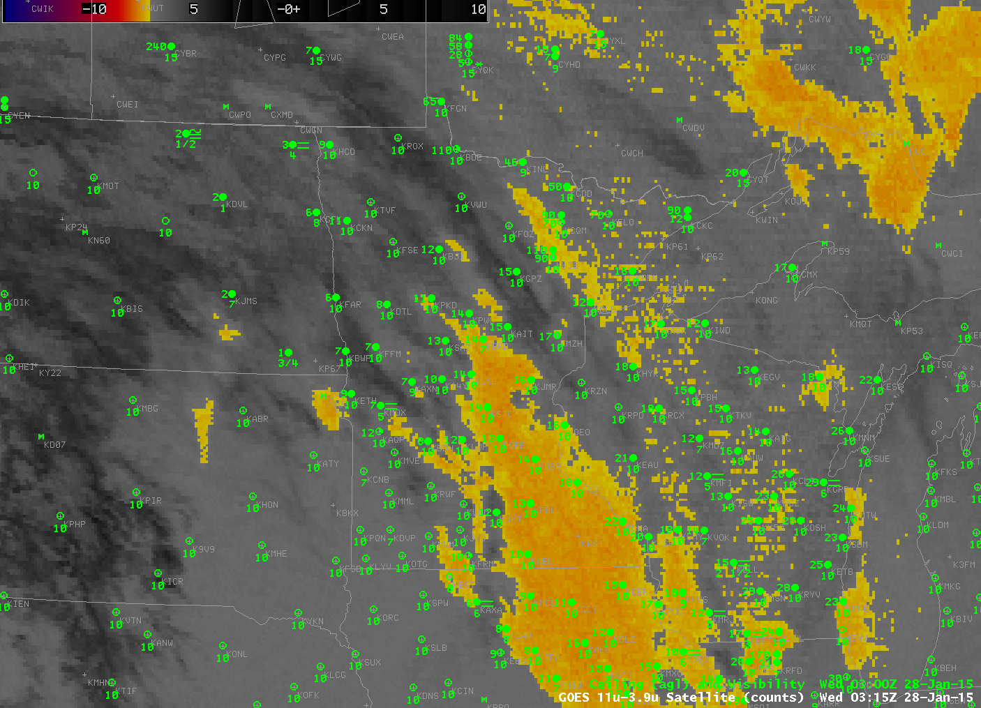
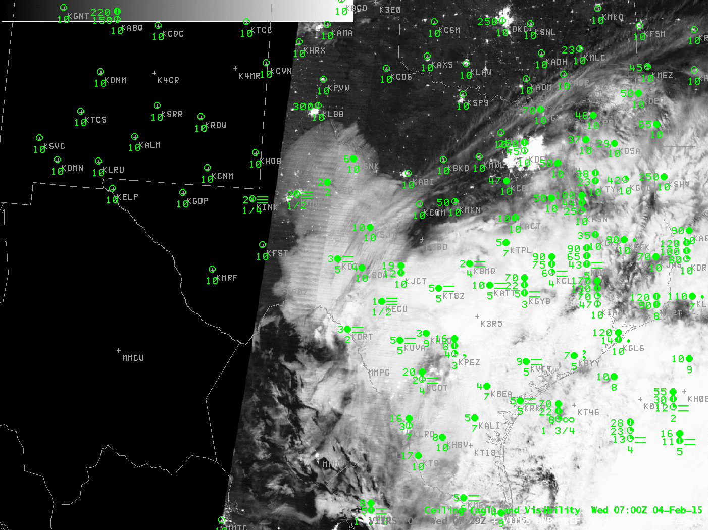
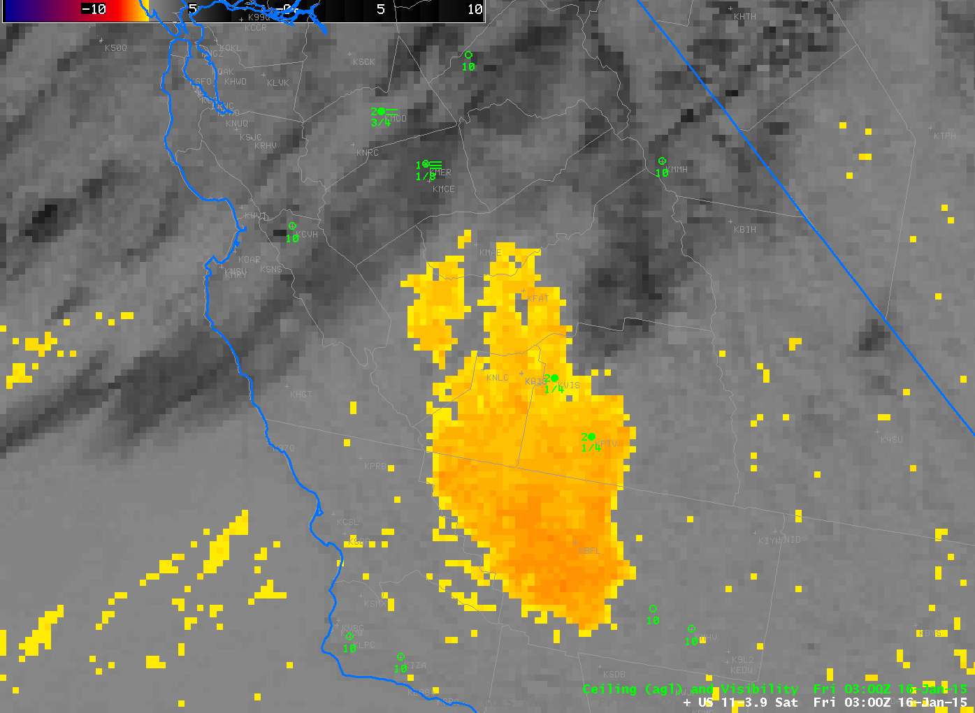
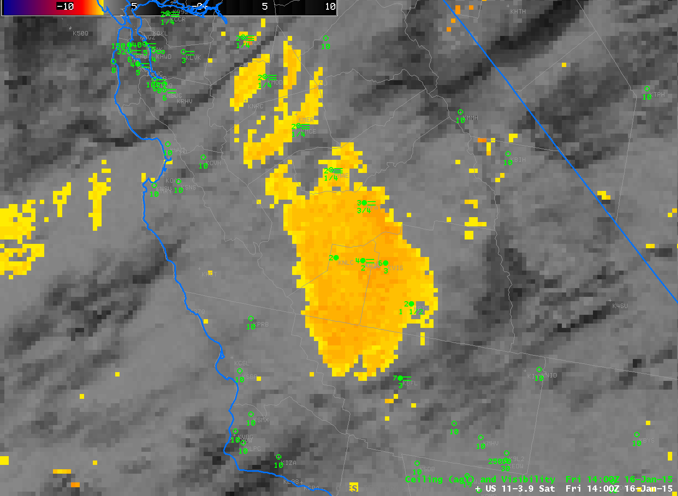
Brightness Temperature Difference (10.7µm – 3.9µm) field from GOES-13, half-hourly from 0315 through 1445 UTC, 28 January 2015, along with surface observations of ceiling and visibility (Click to enlarge)

The traditional method of detecting fog/low stratus is the brightness temperature difference between the shortwave (3.9 µm) and longwave (10.7 µm) infrared channels on GOES. This identification scheme is based on the fact that water droplets do not emit shortwave radiation (3.9 µm) as a blackbody; because of that, the amount of shortwave radiation detected by the satellite is less than it would be if blackboard emissivity were occurring, and the inferred temperature (computed assuming blackboard emission) of the emitting cloud is therefore colder. Water droplets do emit longwave radiation more like a blackbody, so the 10.7 µm brightness temperature is warmer. If the satellite view of low clouds is blocked by cirrus, as above, or by mid-level clouds, then satellite detection of low clouds/fog is hampered or impossible. In the animation above, there are many regions of near-IFR or IFR conditions — low ceilings and reduced visibility — where the Brightness Temperature Difference Product gives no indication that fog/low stratus exists.

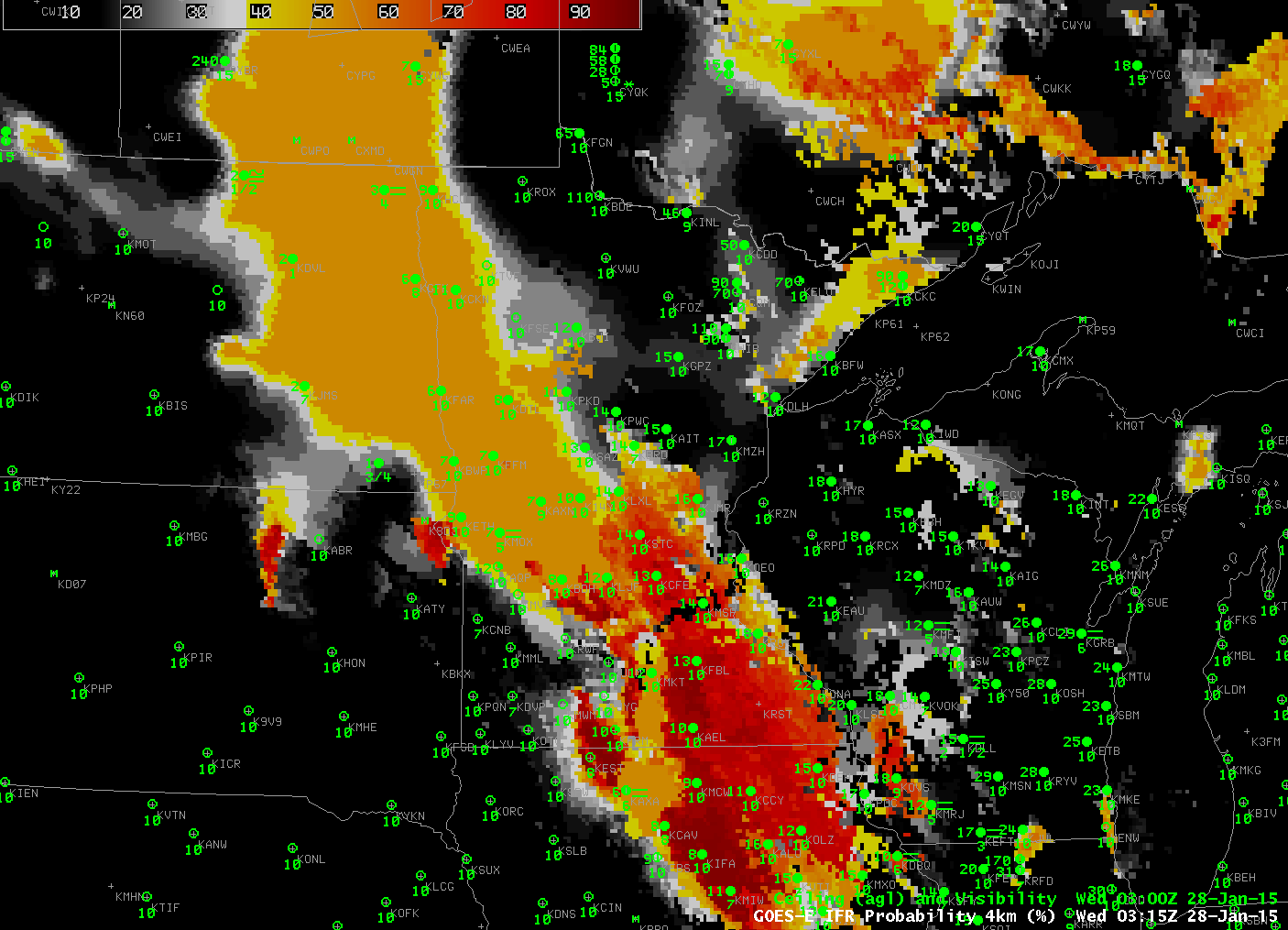
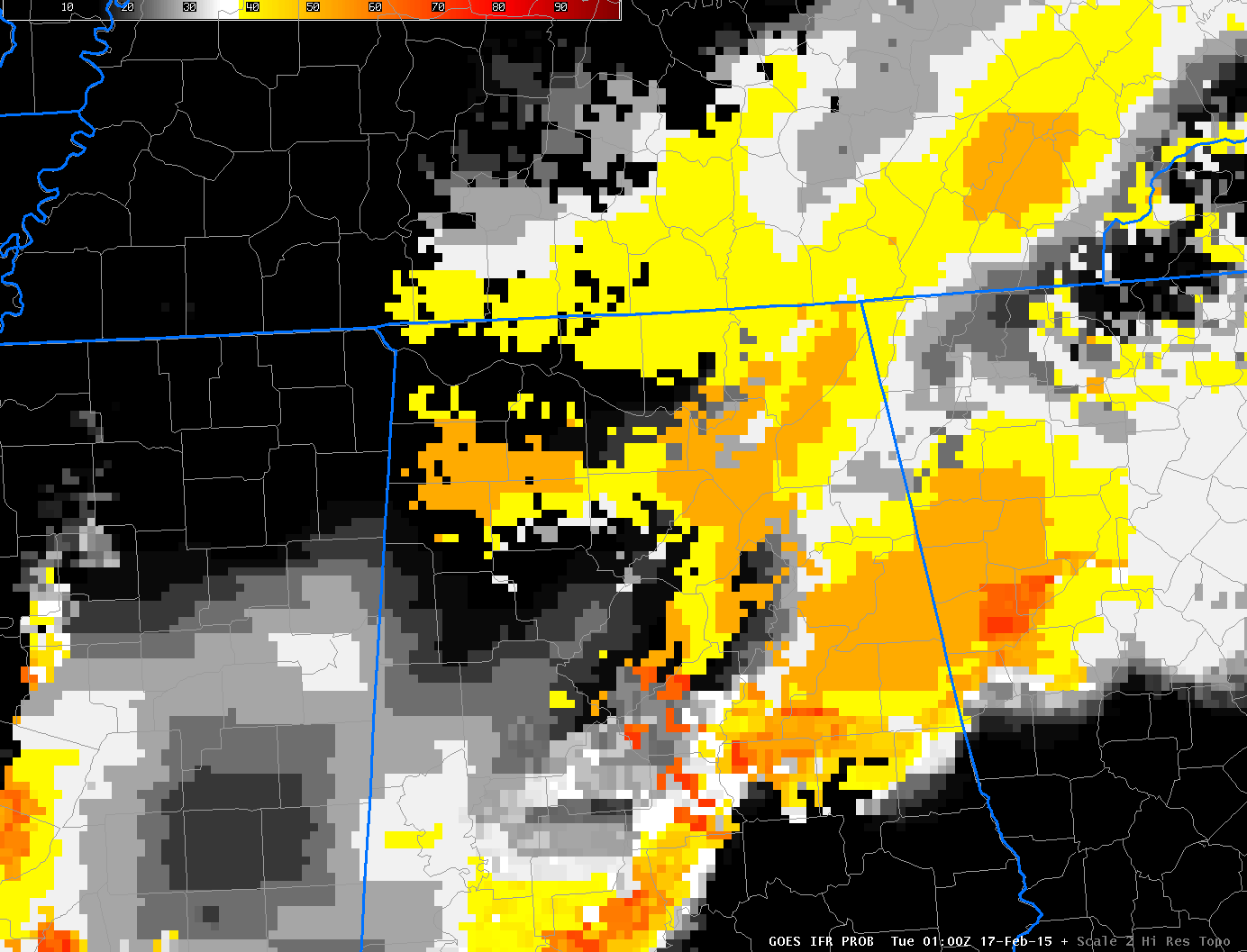
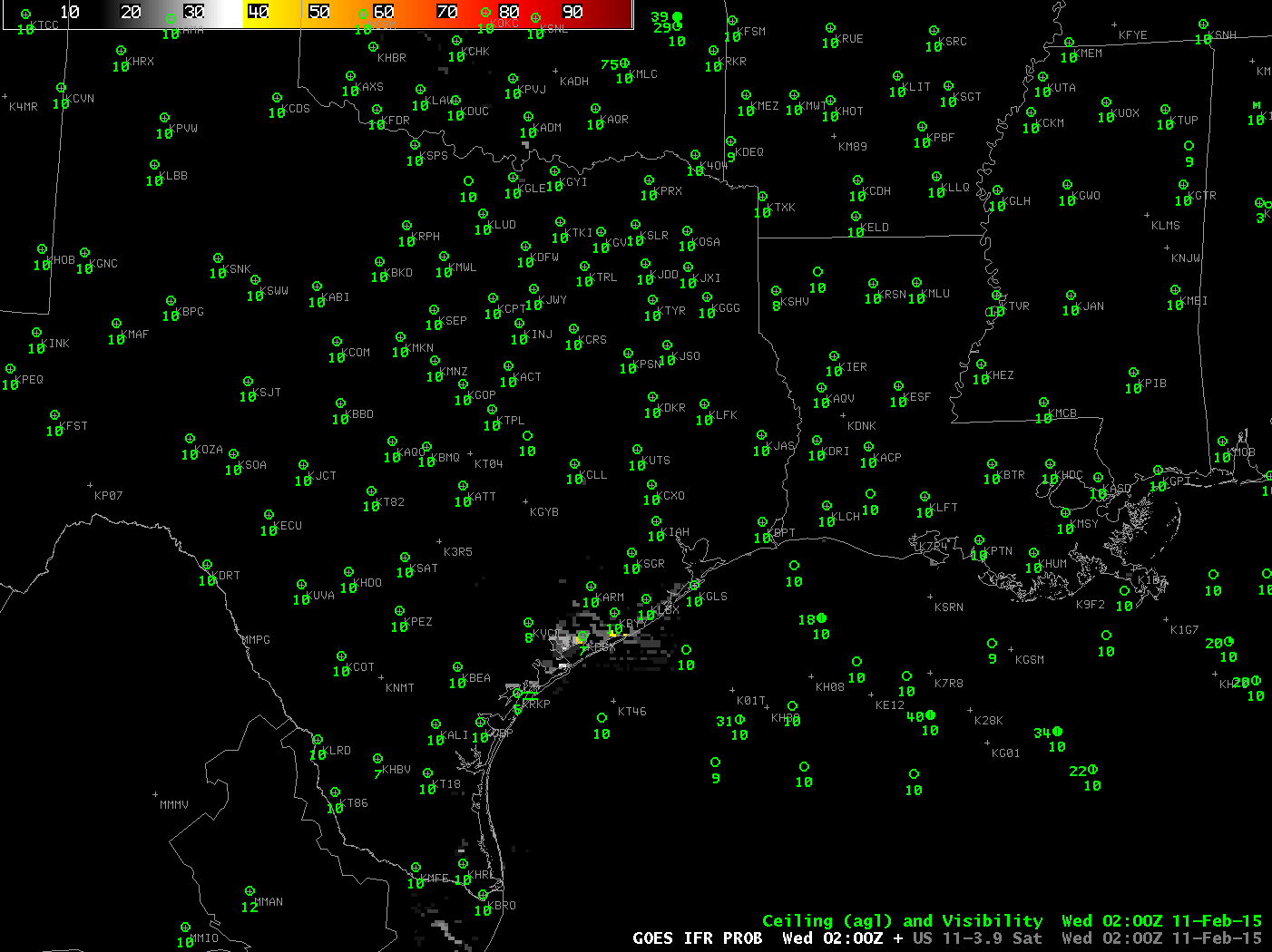
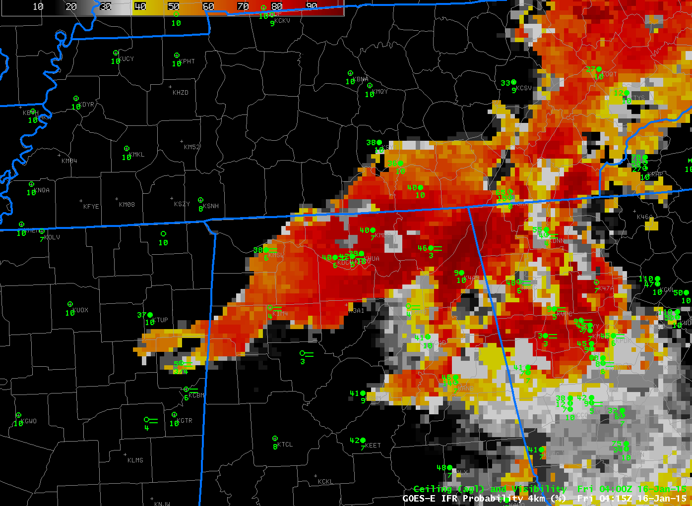
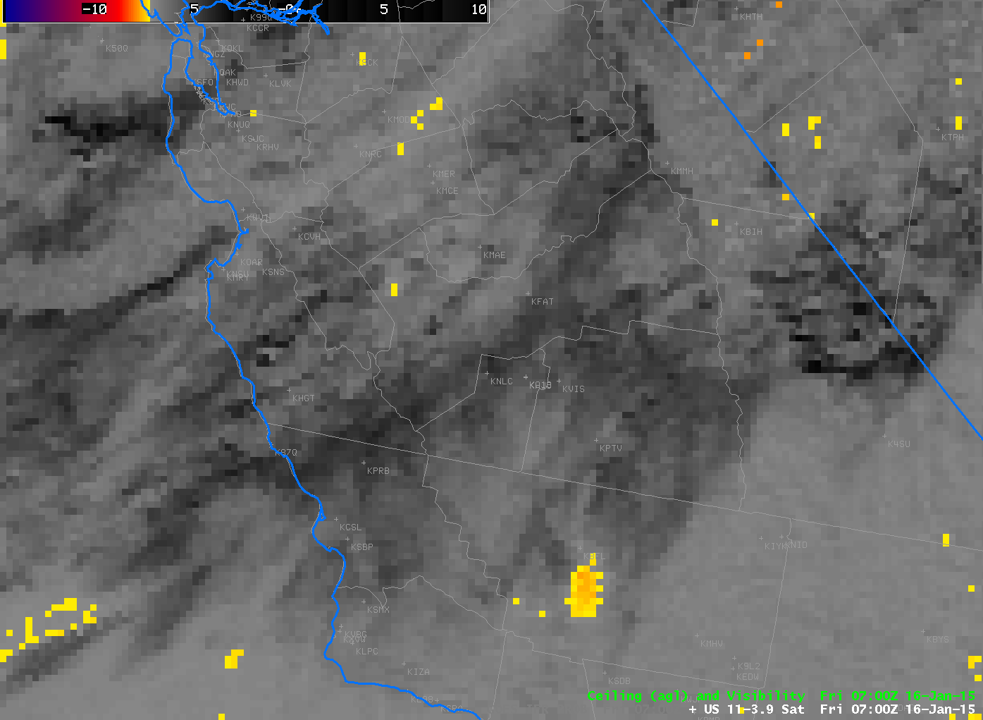
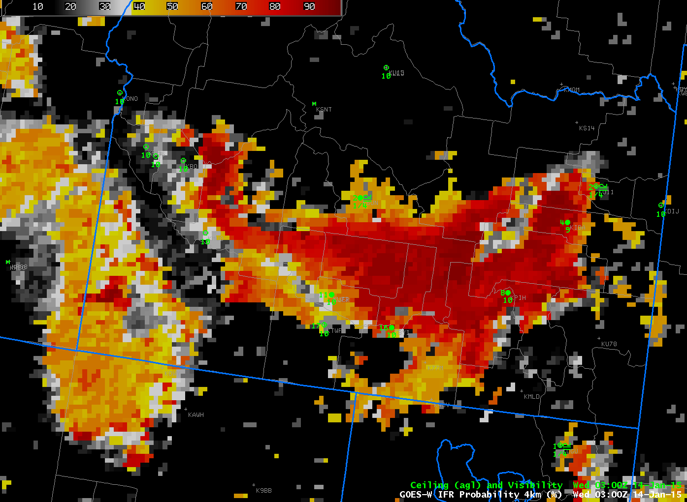
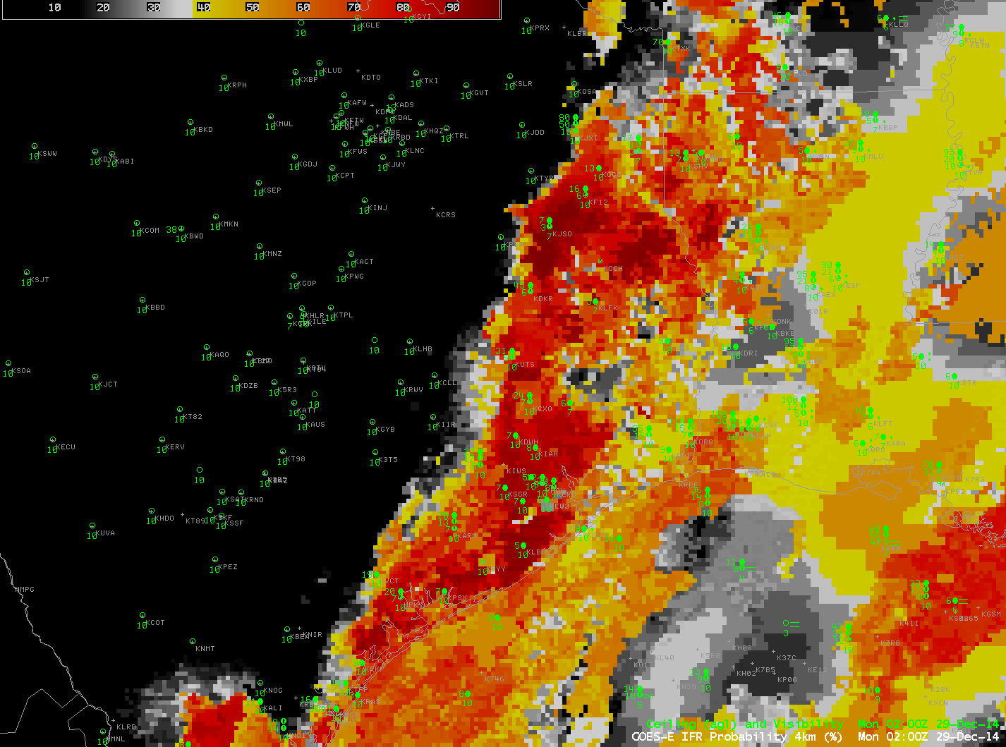
GOES-R IFR Probability fields from GOES-13, half-hourly from 0315 through 1415 UTC, 28 January 2015, along with surface observations of ceiling and visibility (Click to enlarge)

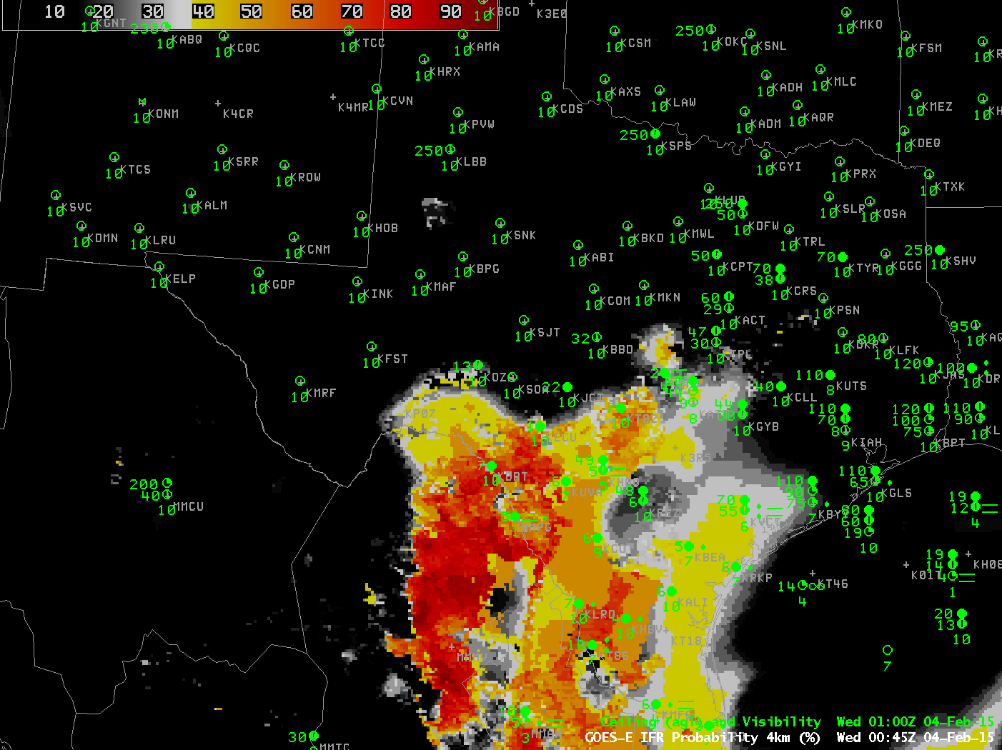
GOES-R IFR Probability fields, above, better capture the horizontal extent of the low ceilings and reduced visibilities. This is because surface data is incorporated into the fields via output from the Rapid Refresh Model output. IFR Probabilities are heightened where the Rapid Refresh Model shows saturation (or near saturation) near the surface, and that includes regions under high/middle clouds, such as the Red River Valley between Minnesota and North Dakota. That model data are controlling the value of the IFR Probability field in those regions is apparent because of two things: (1) The field is horizontally uniform, and not pixelated as it is in regions where higher-resolution satellite data can be used; (2) IFR probability values are smaller because there is less certainty that low clouds are present because the satellite cannot detect them. A well-trained user of this product, then, will interpret IFR Probability values of around 50-60 percent differently in regions of high clouds vs. in regions where low clouds only are present. Note the obvious line in the fields at 1415 UTC — the last image in the animation. This is the boundary between night-time predictors (to the north and west) and daytime predictors (to the south and east). Generally, IFR Probabilities increase as the sun rises because visible satellite data can be used to distinguish between clear and cloudy skies. If there is more certainty that clouds exist, then IFR Probabilities will be greater.

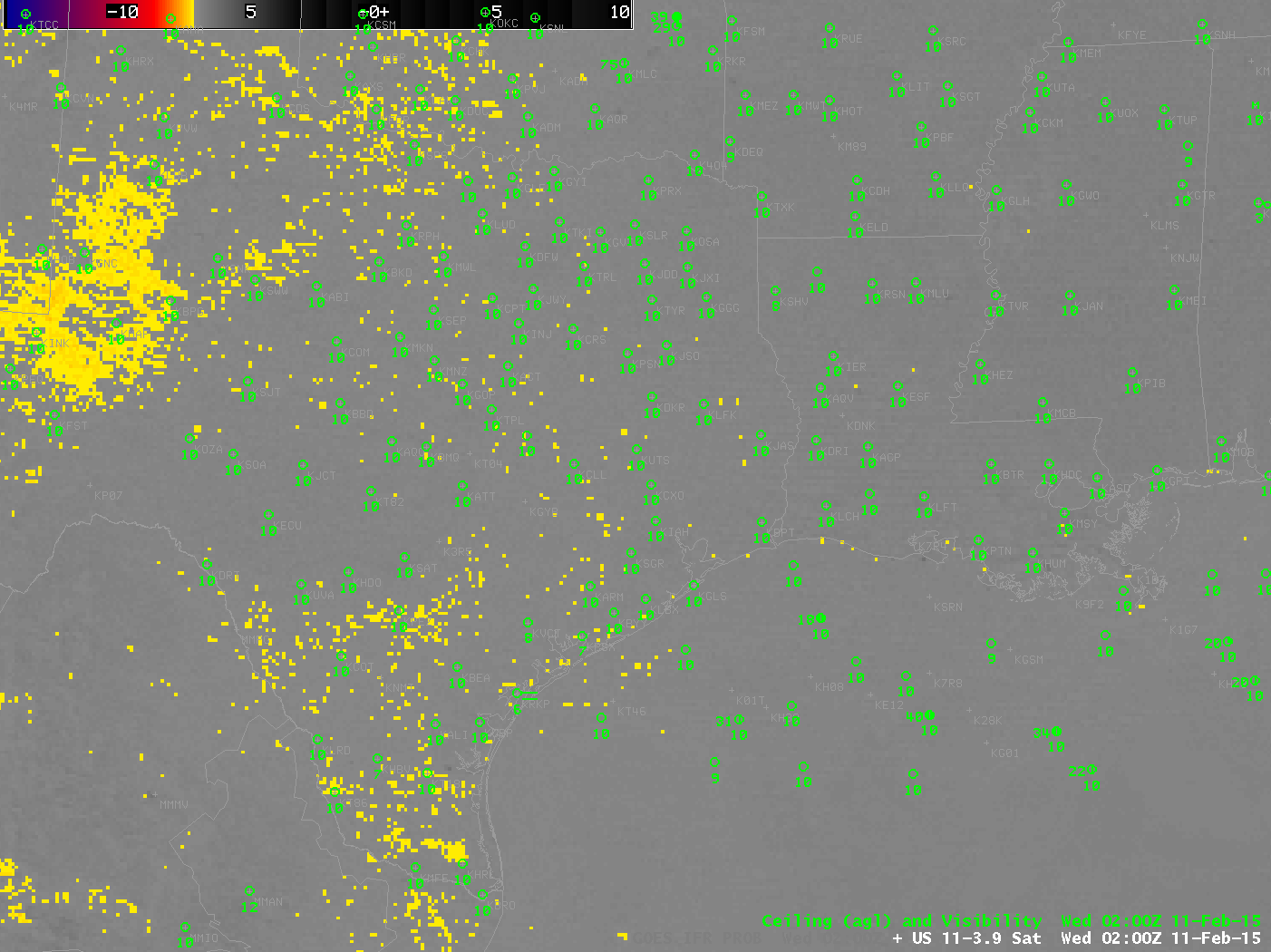
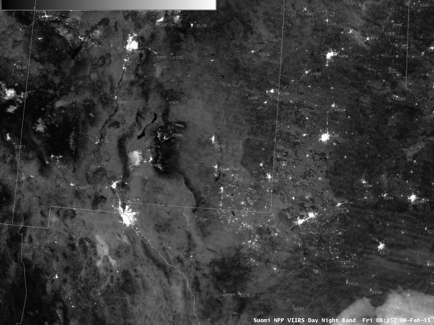
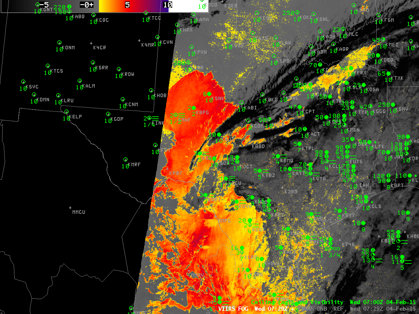
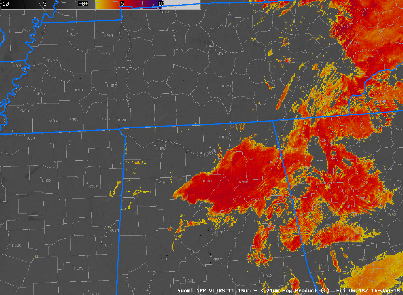
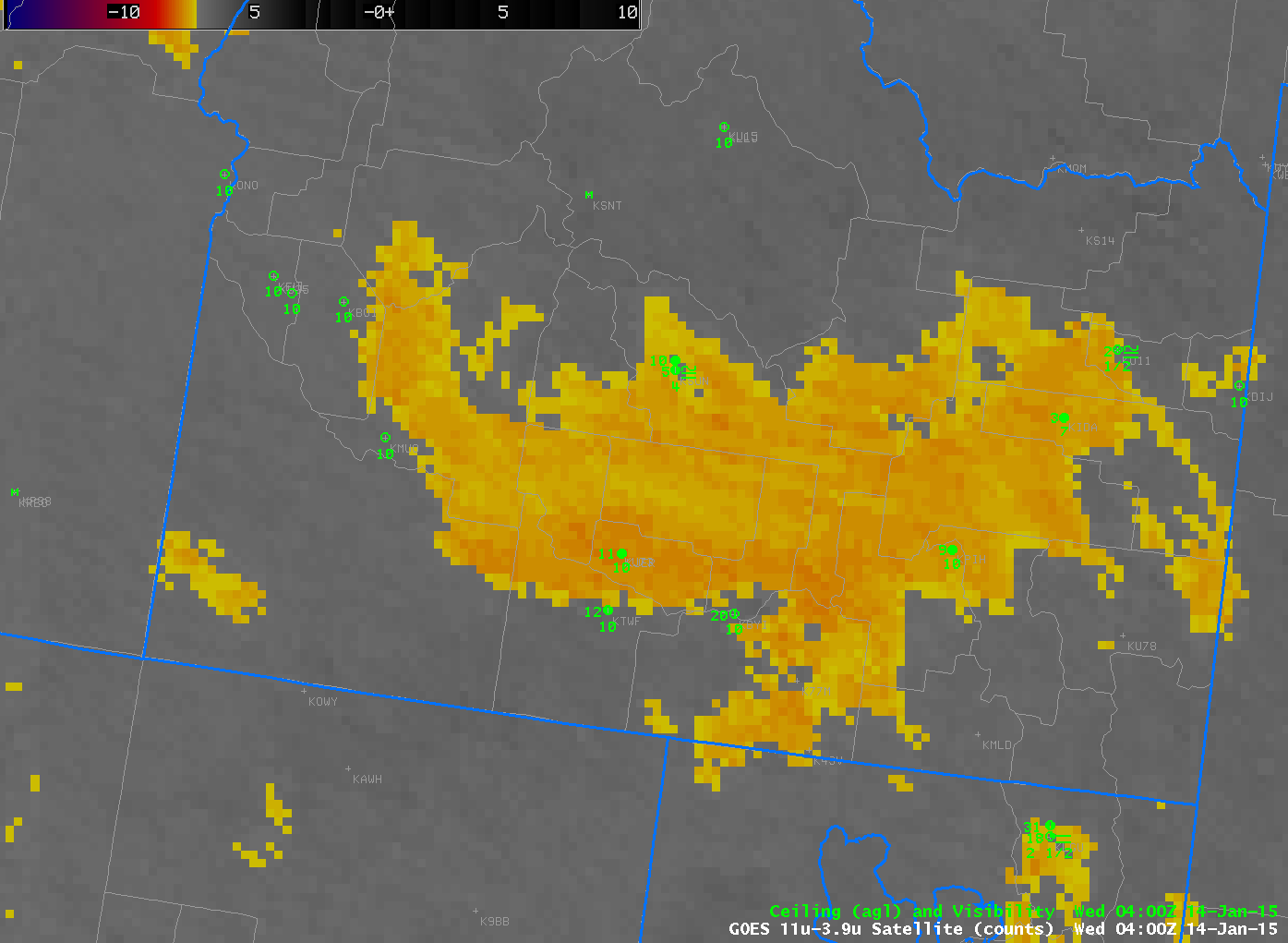
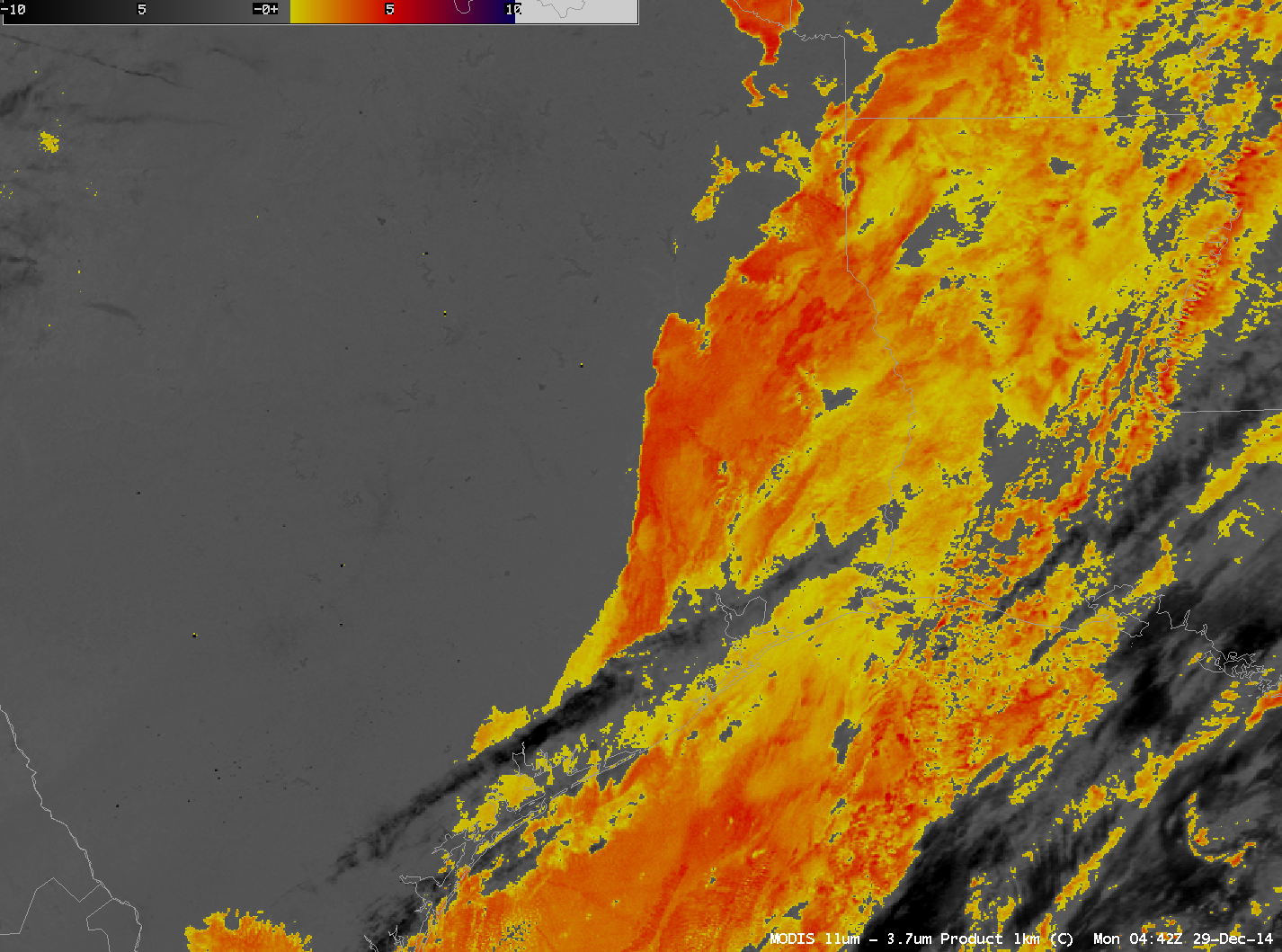
MODIS and Suomi NPP overflew this region and provided information about the clouds. GOES-R IFR Probability is not yet computed using Suomi NPP data; the brightness temperature difference product (11.35 – 3.74), below, shows the widespread cirrus over the region during two sequential overpasses. Scattered breaks allow identification of low clouds. As with any brightness temperature difference product, however, the information is about the top of the cloud, not necessarily the cloud base.

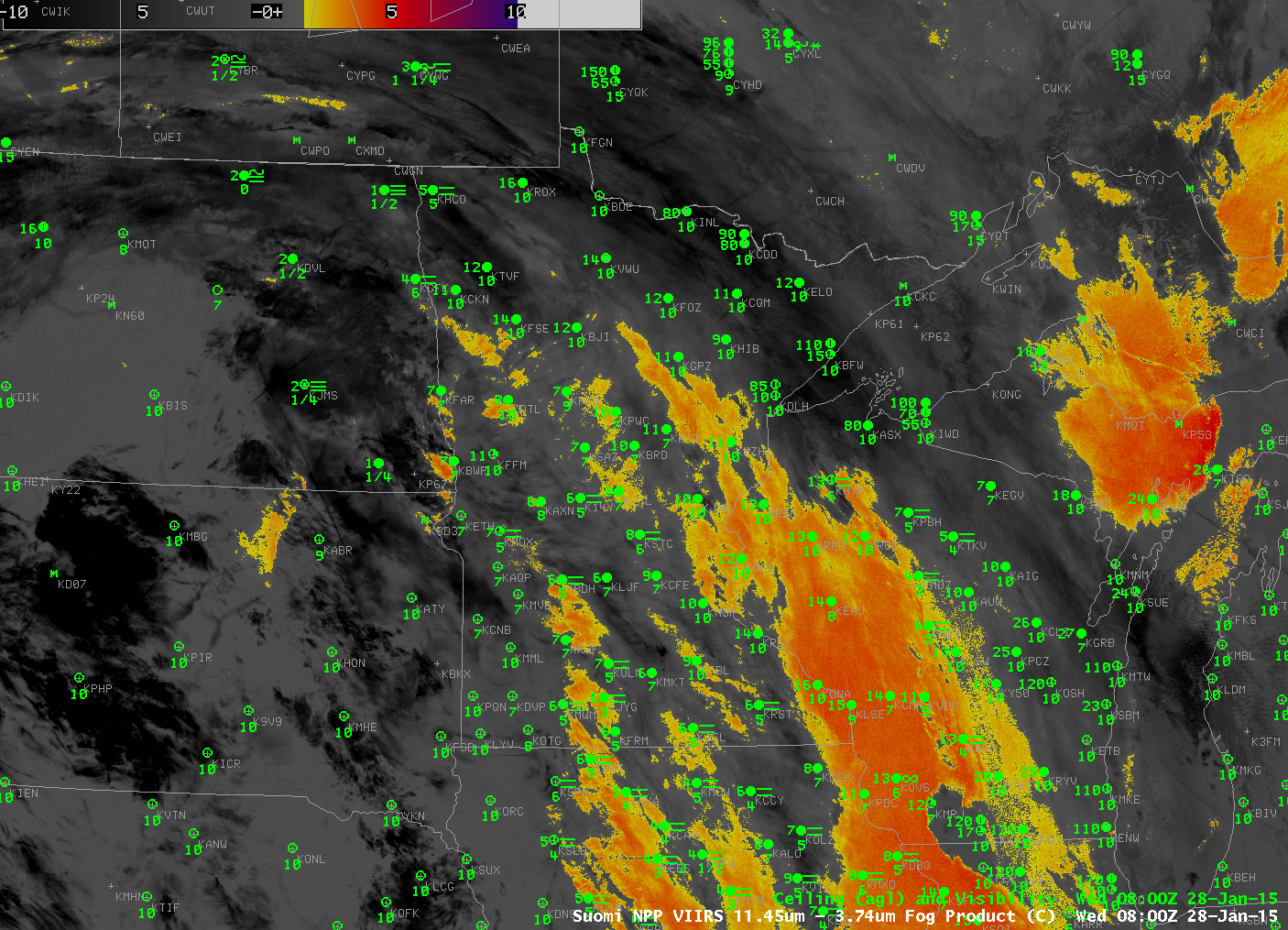
Brightness Temperature Difference (11.35 µm – 3.74 µm) field from Suomi NPP at 0800 and 0941 UTC 28 January 2015, along with surface observations of ceiling and visibility (Click to enlarge)

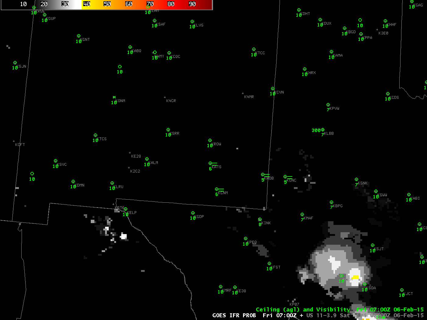
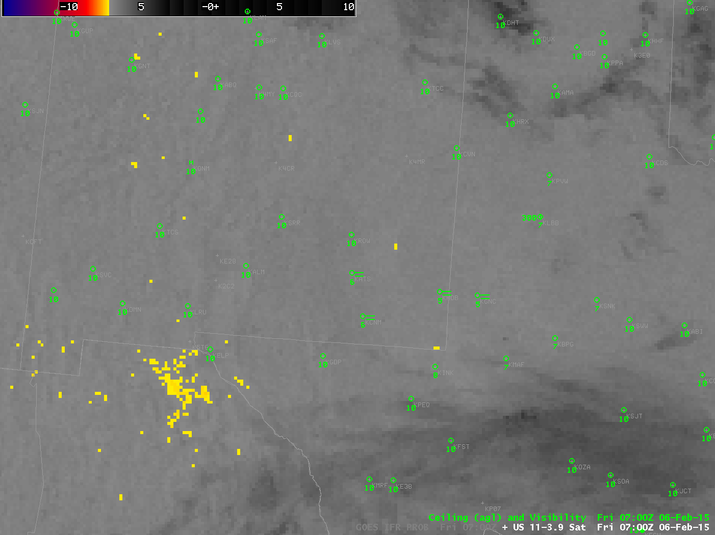
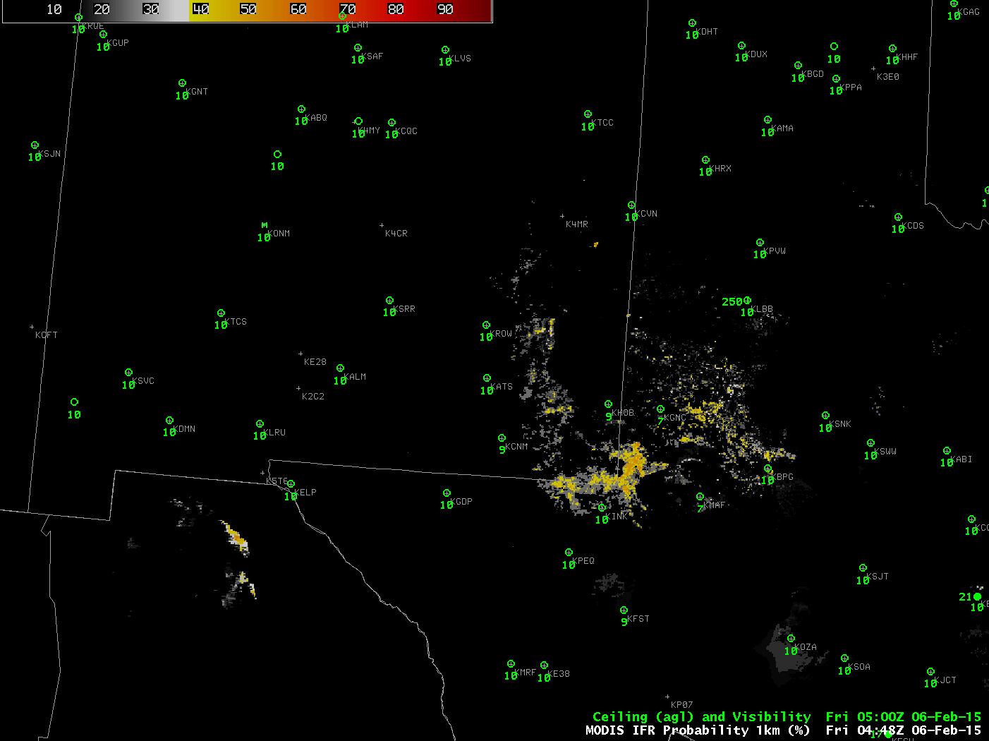
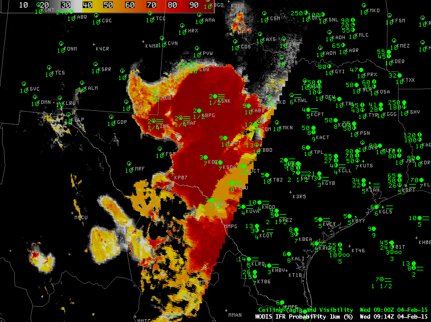
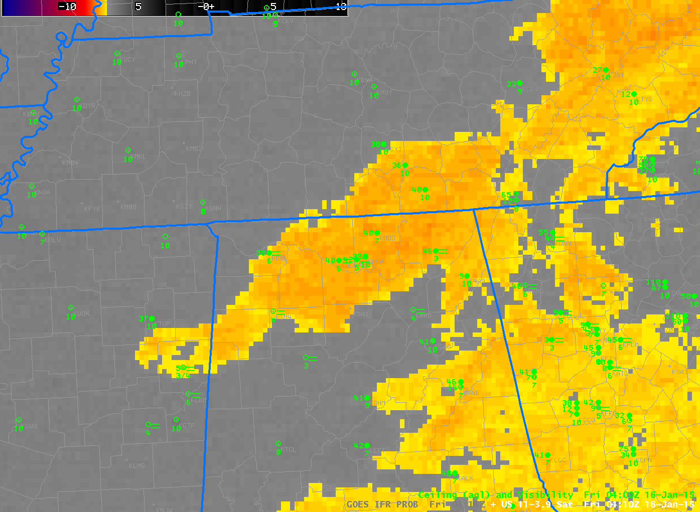
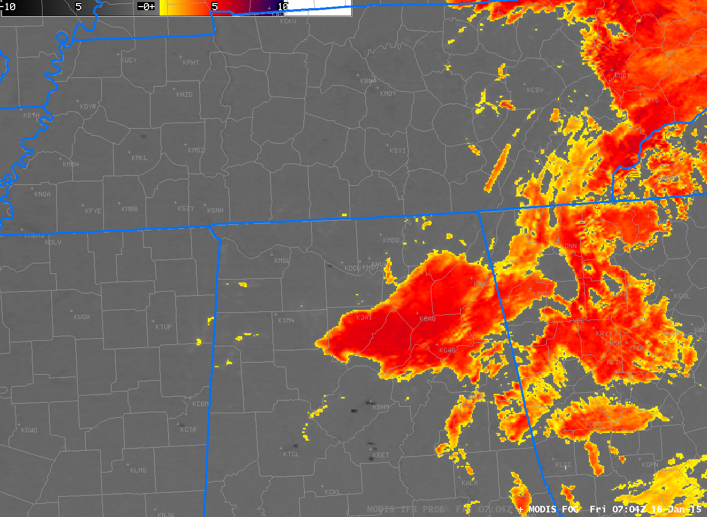
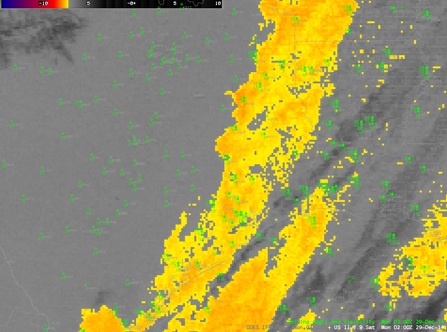
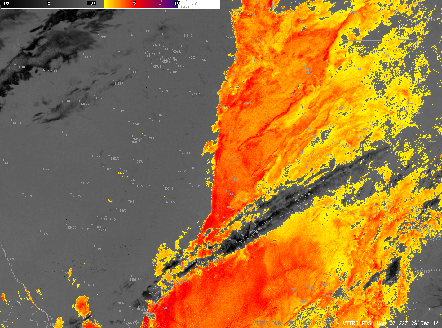
Aqua MODIS estimates of fog are shown below at 0728 and 0907 UTC. Detection using the Brightness Temperature Difference field is hampered by cirrus clouds. IFR Probability fields identify regions under cirrus that show IFR conditions.

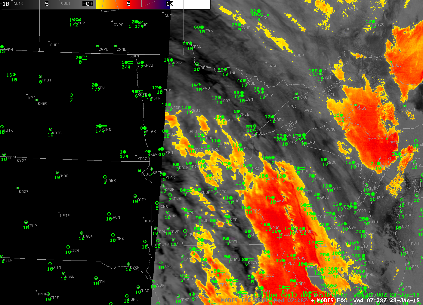
MODIS Brightness Temperature Difference field and MODIS-based GOES-R IFR Probabilities, 0728 UTC 28 January, with surface observations of ceilings and visibility (Click to enlarge)

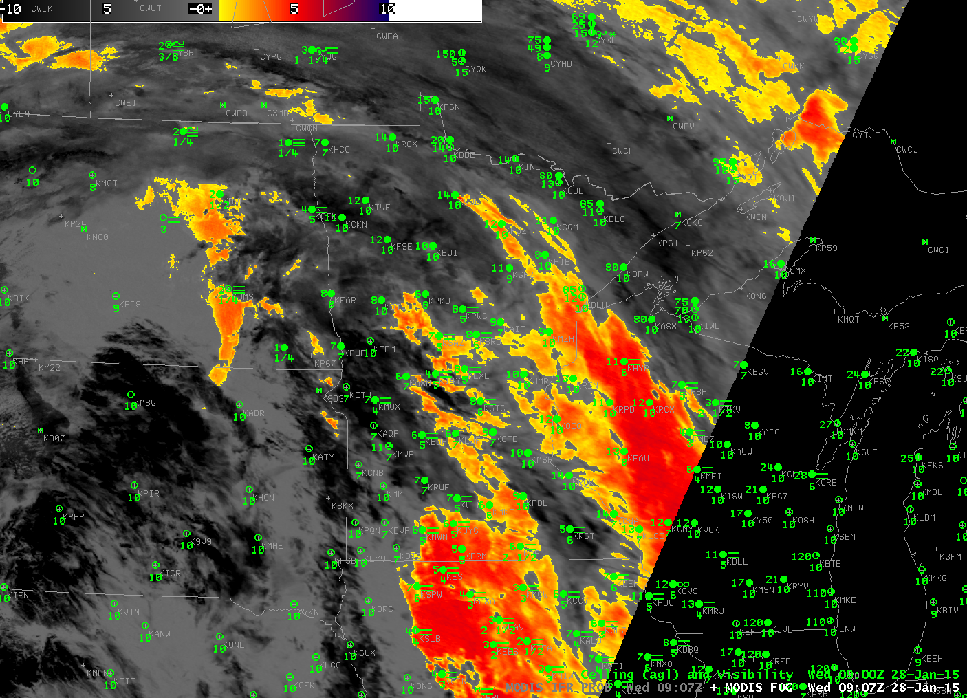
MODIS Brightness Temperature Difference field and MODIS-based GOES-R IFR Probabilities, 0907 UTC 28 January, with surface observations of ceilings and visibility (Click to enlarge)

Using IFR Probability to distinguish between low stratus and mid-level stratus

GOES-based IFR Probability (Upper Left), GOES-13 Brightness Temperature Difference (10.7µm – 3.9µm) (Upper Right), Aqua MODIS-based IFR Probability (Lower Left), Aqua MODIS Brightness Temperature Difference (11µm – 3.7µm) (Lower Right), all with observations of visibility and ceiling, around 0715 UTC 23 January 2015 (Click to enlarge)

The imagery above shows a stratus deck stretching from Wisconsin and Missouri to New York. Both MODIS and GOES Brightness Temperature Difference fields show strong returns that suggest the presence of stratus clouds comprised of water droplets (owing to the difference in emissivity from small droplets at 3.9µm and at 10.7µm). But what about the cloud base, a parameter that is very difficult to determine from satellite data alone?

IFR Probabilities suggest differences in the cloud bases. Highest probabilities are over Wisconsin — where ceilings are around 1000 feet, and where fog is reported (at Lone Rock). Over Indiana and Ohio, IFR Probabilities are low, and ceilings are generally above 2000 feet. IFR Probabilities are higher over Pennsylvania and New York, where ceilings drop again to 600-1000 feet, and where fog is again reported (At Dubois).

The inclusion of surface moisture information (from the Rapid Refresh Model) in the IFR Probability fields allows the IFR Probability fields to better distinguish between low ceilings/fog (known transportation hazards) and higher ceilings in regions of stratus where satellite data alone shows little difference.

Traffic-snarling fog in Huntsville, Alabama

Dense fog developed over the Tennessee River Valley during the morning hours of 16 January 2015, causing crashes and traffic and school delays. The screenshot above (from this link), from WHNT in Huntsville, shows the conditions.

IFR Probability Fields, below, show a large stratus deck moving southward over Alabama, moving south of Hunstville by 0700 UTC. Clear skies allowed additional cooling and a radiation fog developed. The fog impeded transportation in and around Huntsville. IFR Probabilities increased around Huntsville after the large-scale stratus deck moved out, and remained high until around 1500 UTC when all fog dissipated. IFR Probability fields are computed using both satellite data and Rapid Refresh Model data. That IFR Probability is high over Huntsville and surroundings as the fog develops says that satellite data suggests water cloud development and that model data suggests near-surface saturation.

GOES-R IFR Probabilities, half-hourly imagery, 0415-1645 UTC, 16 January 2015 (Click to enlarge)

The fog was also diagnosed using traditional detection methods, such as the brightness temperature difference field from GOES-13 shown below. Brightness Temperature Difference fields detect both fog and elevated stratus, and it’s difficult for satellite data-only products to distinguish between the two cloud types because no surface information is included in a simple brightness temperature difference field.

GOES-13 Brightness Temperature Differences (10.7µm – 3.9µm), half-hourly imagery, 0410-1645 UTC, 16 January 2015 (Click to enlarge)

For a small-scale event such as this, polar orbiting satellites can give sufficient horizontal resolution to give important information. MODIS data from Terra or Aqua can be used to compute IFR Probabilities, and a toggle between the MODIS brightness temperature difference field, and the MODIS-based IFR Probabilities at 0704 UTC is below; unfortunately, Terra and Aqua were not overhead when the fog was at its most dense, but a thin filament of fog/High IFR Probability is developing south of Huntsville in a river valley.

MODIS Brightness Temperature Difference and MODIS-based IFR Probabilities at 0704 UTC on 16 January 2015 (Click to enlarge)

Suomi NPP was positioned such that northern Alabama was viewed on two successive orbits, and the toggle below shows the brightness temperature difference field (11.35 – 3.74). Similar to GOES, Suomi NPP Brightness Temperature Difference fields show the development of water-based clouds in/around Huntsville.

Suomi NPP Brightness Temperature Difference fields at 0645 and 0828 UTC, 16 January 2015 (Click to enlarge)

When Cirrus overlies Fog

GOES-15 Visible Imagery at 1800 UTC on 12-15 January 2015 (Click to enlarge)

Fog and low stratus has persisted in California’s central valley during the week of 12-16 January 2015. The visible imagery above shows the extent of the fog/low stratus at 1800 UTC on 12-15 January.

During the early morning hours of 16 January, high cirrus started to overspread the central Valley (That cirrus is apparent in the visible iamgery from 15 January above). The presence of cirrus makes use of the traditional method of fog detection — brightness temperature difference — problematic because the satellite no longer senses radiation from the low clouds; rather, cirrus radiation is being detected.

The four toggles below show Brightness temperature Difference and GOES-R IFR Probabilities at 0300 (top), 0700 (second from top), 1100 (second from bottom) and 1400 UTC (bottom) on 16 January 2015. At 0300 UTC, cirrus has overspread the northern part of the central Valley. At this time Merced, CA, shows IFR conditions. IFR Probabilities under the cirrus there show a flat field characteristic of conditions when IFR Probabilities are governed by Rapid Refresh data only. Probabilities are higher where satellite data are also included as predictors.

At 0700 UTC and 1100 UTC, cirrus has overspread the entire valley (with occasional breaks). Values of GOES-R IFR Probability are therefore suppressed, so interpretation of the IFR Probability value should be tempered by knowledge of the cloud field. A low value under clear skies means something different than a low value under a cirrus canopy. Under a cirrus canopy, the accuracy of the GOES-R IFR Probability Field depends on the accuracy of the Rapid Refresh model.

AT 1400 UTC, as the cirrus shield retreats, IFR Probabilities increase again over the central Valley.

Toggle between GOES-R IFR Probabilities from GOES-15 and Brightness Temperature Difference Fields, 0300 UTC 16 January 2015 (Click to enlarge)

Toggle between GOES-R IFR Probabilities from GOES-15 and Brightness Temperature Difference Fields, 0700 UTC 16 January 2015 (Click to enlarge)

Toggle between GOES-R IFR Probabilities from GOES-15 and Brightness Temperature Difference Fields, 1100 UTC 16 January 2015 (Click to enlarge)

Toggle between GOES-R IFR Probabilities from GOES-15 and Brightness Temperature Difference Fields, 1400 UTC 16 January 2015 (Click to enlarge)

Freezing Fog over Idaho’s Snake River Valley

GOES-R IFR Probabilities over southern Idaho, hourly from 0300 through 1800 UTC on 14 January 2015 (Click to enlarge)

High Pressure over the Rocky Mountains, and its associated inversion, has trapped moisture at low levels, including along the Snake River in southern Idaho. As a consequence, fog is prevalent at low levels, and cold temperatures are allowing for the development of freezing fog. (Click here for a National Weather Service advisory from the Pocatello WFO).

The GOES-R IFR Algorithm shows high probabilities over the Snake River Valley where the Fog/Freezing Fog was occuring — Twin Falls and Rexburg both reported freezing fog during the animation above. The Brightness Temperature Difference field, below, also captures the areal extent of the low stratus deck.

GOES Brightness Temperature Difference fields (10.7µm – 3.9µm) over southern Idaho, hourly from 0400 through 1800 UTC on 14 January 2015 (Click to enlarge)

Sharp edge to Fog/Low Stratus over east Texas

Brightness Temperature Difference Fields (10.7µm – 3.9µm) and surface observations of ceilings and visibilities, Hourly from 0200 through ~1400 UTC [Click to enlarge].

Traditional method of fog/low stratus detection revealed a sharp edge to clouds over east Texas during the morning of 29 December 2014. The animation above reveals several difficulties inherent in using brightness temperature difference fields in diagnosing fog/low stratus. Where multiple cloud layers are present — such as along the coast at 0500-0600 UTC — the brightness temperature difference product cannot view the low clouds. At sunrise, increasing amounts of solar 3.9µm radiation causes the brightness temperature difference product to flip sign. The signal for low clouds is still there, however.

GOES-R IFR Probabilities and surface observations of ceilings and visibilities, Hourly from 0200 through ~1400 UTC [Click to enlarge]

The animation of GOES-R IFR Probabilities, above, created from GOES-13 data and Rapid Refresh Model data, shows high IFR Probabilities over east Texas where low ceilings and reduced visibilities prevailed, including metropolitan Houston. The algorithm suggests the likelihood of fog/low stratus underneath the cirrus debris that is over the coast around 0500-0600 UTC as well, because the Rapid Refresh model output in that region strongly suggests low-level saturation. In addition, the fields show only minor changes through sunrise (the effect of the terminator is present in the final image in the loop).

MODIS data from either Terra or Aqua can be used to produce IFR Probabilities. The data below is from 0442 UTC. Polar orbiter data is infrequent, however, so temporal monitoring of the fog/low clouds is more easily achieved using GOES data. MODIS data, like the GOES data above, shows the effects of cirrus clouds on Brightness Temperature Difference fields and on IFR Probabilities. Cloud predictors of low clouds/fog from satellite cannot be used in regions of cirrus, so IFR Probabilities are smaller in regions where multiple cloud layers exist, which regions are where only Rapid Refresh Data can be used as predictors.

0442 UTC MODIS-based brightness temperature difference and IFR Probability fields (Click to enlarge)

Brightness Temperature Difference fields can also be created from Suomi/NPP data and the orbital geometry on 29 December meant that eastern Texas was viewed on two sequential overpasses. IFR Probabilities are not quite yet computed using Suomi NPP data, but the brightness temperature difference fields can be used to show where water-based clouds exist. They show a very sharp western edge to the clouds.

Brightness Temperature Difference Fields (11.35µm – 3.74µm) from Suomi NPP at 0723 and 0904 UTC on 29 December 2014 (Click to enlarge)

The Day Night Band on Suomi NPP produces visible imagery at night. When lunar illumination is strong, it can provide compelling imagery. On 29 December 2014, however, the moon set around 0600 UTC, so no lunar illumination was available, and fog/low clouds are very difficult to discern in the toggle below between the Day Night Band and the brightness temperature difference field at 0723 UTC.

Day Night Band and Brightness Temperature Difference Fields (11.35µm – 3.74µm) from Suomi NPP at 0723 on 29 December 2014 (Click to enlarge)

GOES-R Fog Product Examples

Fog detection fusing GOES, Terra/Aqua or Suomi/NPP Satellite data with Model output