Category Archives: Suomi/NPP

Fog over snow in the upper midwest

Suomi/NPP Brightness Temperature Difference (11.35 µm – 3.74 µm) Brightness Temperature Difference and Day/Night Band, 0840 UTC 27 December 2013 (click image to enlarge)

At times of low lunar illumination, it can become increasingly difficult to discern regions of clouds and snow in the Suomi/NPP day/night band, shown above, toggling with the brightness temperature difference. Nevertheless, careful perusal of the image reveals cloud edges over northeastern Wisconsin and through central lower Michigan that are confirmed by the brightness temperature difference field. In contrast, the whiter region that stretches southwestward from Des Moines towards extreme northeastern Kansas has no signal in the brightness temperature difference field. This is snow on the ground (vs. little snow to the northwest).

GOES IFR Probabilities computed with GOES-13 data, hourly from 0615 UTC through 1302 UTC, 27 December 2013 (click image to enlarge)

IFR Probability fields and GOES-Based brightness temperature difference fields are produced to aid in the detection of low clouds. In the animation above, higher IFR probabilities are centered on north-central Wisconsin where, intially, IFR conditions are not quite met (according to the plotted observations of ceiling and visibilities). However, as the night progresses, ceilings lower and visibilities decrease as IFR conditions do develop in regions where IFR Probabilities are high. The IFR probabilities roughly overlap the region where IFR conditions exist.

Note that encroachment of higher clouds in from the west, starting around 0800 UTC, means that satellite data cannot be used in the IFR Probability algorithm. Because only model data are used, IFR probabilities drop from values at/above 80% to values between 50 and 60% even as IFR conditions come to be more widespread. For this reason, it is important when interpreting IFR Probabilities to be alert to the presence of high clouds.

IFR Probabilities give a much more better approximation of where fog/low stratus may be occurring than a simple brightness temperature difference field. The toggle between the GOES-R IFR Probabilities and the GOES-13 Brightness Temperature Difference, below, gives testimony to this.

Fog Detection under Cirrus

GOES-R IFR Probabilities from GOES-13 (Upper Left), GOES-13 Brightness Temperature Difference Product (10.7 µm – 3.9 µm) (Upper Right), GOES-R Cloud Thickness from GOES-13 (Lower Left), MODIS-based IFR Probabilities (Lower Right), Times as indicated (click image to enlarge)

Dense Fog developed over the southern Plains overnight, and the case demonstrates how the Fused data product is able to give a useful signal of IFR probabilities even in regions where high clouds preclude the detection of low clouds by satellite. The fog was widespread and dense enough to warrant Dense Fog Advisories from Tulsa, Norman and Topeka forecast offices. See below, for example.

000
FXUS64 KTSA 020953
AFDTSA

AREA FORECAST DISCUSSION
NATIONAL WEATHER SERVICE TULSA OK
353 AM CST MON DEC 2 2013

.DISCUSSION…
DENSE FOG CONTINUES THIS MORNING ACROSS MUCH OF THE CWA. GIVEN THE
TIME OF YEAR /LOW SUN ANGLE/ AND THE FACT THAT SOME HIGH CLOUDS ARE
STREAMING INTO THE AREA FROM THE NW /REDUCED INSOLATION AND
DELAYED MIXING/…THINK IT MAY TAKE A LITTLE LONGER THAN
PREVIOUSLY EXPECTED TO GET RID OF THE FOG. WE HAVE EXTENDED THE
DENSE FOG ADVISORY UNTIL 11 AM. ONCE THE FOG BURNS OFF…SHOULD
BE A PLEASANT DAY WITH UNSEASONABLY WARM TEMPS AND FAIRLY LIGHT
WIND. COULD BE SOME MORE FOG TUESDAY MORNING IN SOME PLACES BUT A
LITTLE MORE WIND MAY KEEP IT FROM GETTING AS DENSE AND AS
WIDESPREAD AS IT IS THIS MORNING. SLIGHTLY WARMER TEMPS IN STORE
TUESDAY WITH SOME PLACES LIKELY IN THE 70S. WARM AND WINDY
CONDITIONS WILL RESULT IN AN INCREASING FIRE WEATHER CONCERN.

Satellite detection of this fog event was constrained by the presence of two upper-level cloud decks. At the beginning of the animation, above, high clouds associated with the subtropical jet are over the southern quarter of the domain plotted. These high clouds quickly shift southward, and the region in the brightness temperature difference product that is consistent with detection of fog/low stratus (that is, low water-based clouds) expands to the south (surface observations suggest the low stratus clouds were present earlier, but masked by the higher clouds). Later in the animation, high clouds sag southward into the northern part of the domain. When this happens, low stratus/fog (indicated in observations by IFR conditions) are not detected by GOES because the higher ice clouds block the view of the scene. However, the IFR Probability fields that use both satellite data and output from the Rapid Refresh Model continue to depict a likely region (confirmed by the observations) of reduced visibilities. IFR Probabilities do drop, of course, as satellite data cannot be used to confirm the presence of low clouds. Knowledge of why the probabilities drop is vital to the interpretation of the field: You have to know that the high clouds are present, either by looking at the satellite data, or by understanding that the character of the IFR Probability field changes to one that is less pixelated when satellite data cannot be included because of ice clouds above the low stratus deck.

For a large-scale event like this, MODIS-based IFR Probabilities overlap well with GOES-Based IFR Probabilities, as shown in the image above. In cases like this sometimes individual river valleys will show up with slightly elevated IFR Probabilities (or cloud thicknesses).

The GOES-R Cloud Thickness field is computed for the highest water-based cloud detected (during non-twilight conditions — that is, not during the hour or so surrounding sunrise and sunset). Note how well the thickest clouds — over northeast OK, surrounding Tulsa — correlate with the strongest Brightness Temperature Difference, both in GOES and in Suomi/NPP data (below). Note also how the Cloud Thickness field is not computed in regions where higher ice-based clouds are present.

GOES-R IFR Probabilities from GOES-13 (Upper Left), GOES-13 Brightness Temperature Difference Product (10.7 µm – 3.9 µm) (Upper Right), GOES-R Cloud Thickness from GOES-13 (Lower Left), Suomi/NPP Brightness Temperature Difference from VIIRS (10.35 µm – 3.74 µm) (Lower Right), Times near 0802 UTC as indicated (click image to enlarge)

Cloud Thickness can be used to predict the time of fog dissipation, using this scatterplot/relationship. If sun angle is limited by the season, or if solar insolation is limited by higher clouds, you might adjust the first guess for dissipation to a later time.

A Reminder about Co-Registration Errors

GOES-R IFR Probabilities from GOES-13, times as indicated on 27 November 2013 (click image to enlarge)

The GOES-R IFR Probability field showed enhanced probabilities surrounding lakes and rivers in Louisiana and Texas overnight. This is in large part due to a strong signal in the Brightness Temperature Difference field. There is a co-registration error between the 10.7 µm and 3.9 µm detectors on the GOES Imager. This means that the pixel locations for the two channels are not aligned, and at times the mis-alignment is large enough that a fog signal is produced. In the present case, one of the detectors sees the warm waters of a lake, and the second detector sees the adjacent (much cooler) shoreline, but the navigation misalignment is such that both pixels are believed to be co-located. Thus a difference in the brightness temperature occurs not because of emissivity difference properties in clouds (which also makes the 3.9 micron brightness temperature appear cooler) but because of a co-registration error. The brightness temperature difference field from 0802 UTC is below (the 0745 UTC image is very similar). Note how the enhanced brightness temperature difference field appears to have a shadow just to its west. It is possible for this to occur if a cloud is forming downwind of a warm lake. However, in the present case, winds were primarily northerly, not westerly.

GOES-13 Brightness Temperature Difference Product (10.7 µm – 3.9 µm) 0802 UTC 27 November 2013 (click image to enlarge)

Polar Orbiting satellites viewed this region contemporaneously. Aqua, carrying the MODIS instrument, passed overhead at 0745 UTC, and Suomi/NPP at 0802. What did they see? The 3.9 µm channel from MODIS, below, highlights the warm lake waters over eastern Texas and Louisiana. There is little indication in this image of clouds near the lakes.

MODIS Brightness temperature at ~3.9 µm 0802 UTC 27 November 2013 (click image to enlarge)

The brightness temperature difference product from MODIS, below, and the MODIS-based IFR Probabilities also show no indication of fog/low stratus near the bodies of water in east Texas/Louisiana.

MODIS Brightness temperature difference (11.0 µm – 3.9 µm) and MODIS-based IFR Probabilities at 0746 UTC 27 November 2013 (click image to enlarge)

Suomi/NPP data are shown below. The Brightness Temperature Difference (10.35 µm – 3.74 µm) Field, the 3.74 µm field and the Day/Night band all are consistent with clear skies near the water bodies of east Texas and western Louisiana.

Suomi/NPP VIIRS Brightness Temperature Difference (10.35 µm – 3.74 µm) and Day/Night band at 0802 UTC 27 November 2013 (click image to enlarge)

Be cautious when interpreting the brightness temperature difference from GOES (and IFR Probabilities that are computed using the satellite signal) along land/water boundaries. GOES Engineers continue to investigate methods of mitigating this co-registration error.

Fog and Stratus in the Southeast United States

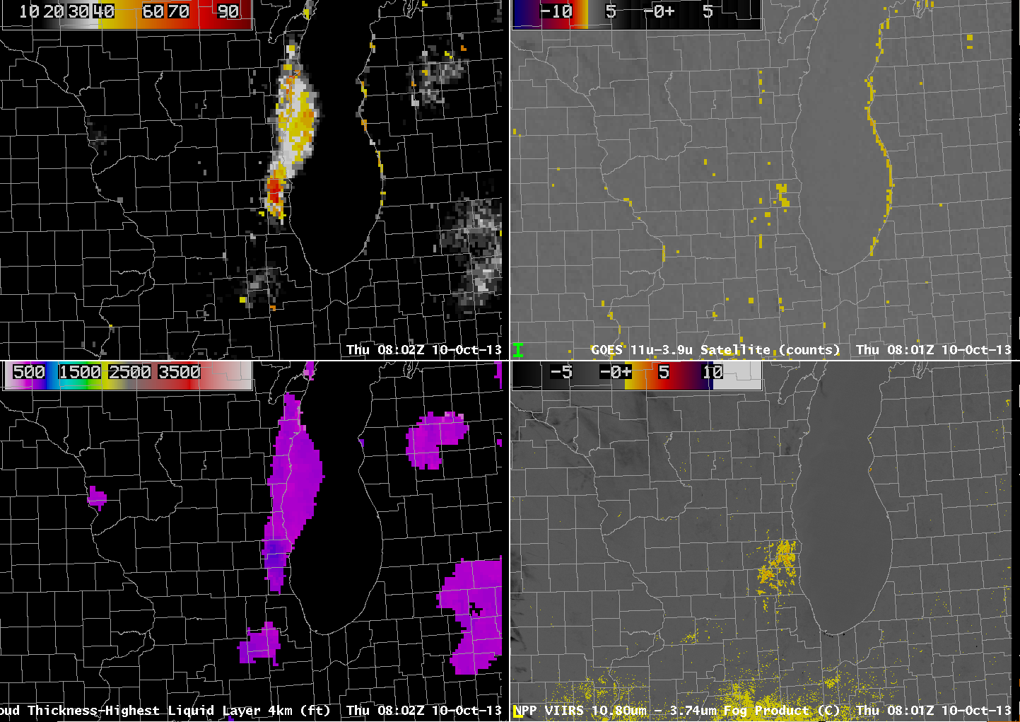
Fog and Stratus with IFR Conditions developed along the Southeast Coast of the United States on the morning of November 22. In some places, the GOES-IFR Probability fields gave a signal of the developing visibility obstructions more than an hour before the traditional brightness temperature difference signal. At 0202 UTC, below, the IFR Probability fields suggest a continuous region of enhanced probabilities of IFR conditions developing along the South Carolina coastline. Both IFR Probabilities and the brightness temperature difference fields agree that Fog/Low Stratus are already present over coastal North Carolina.

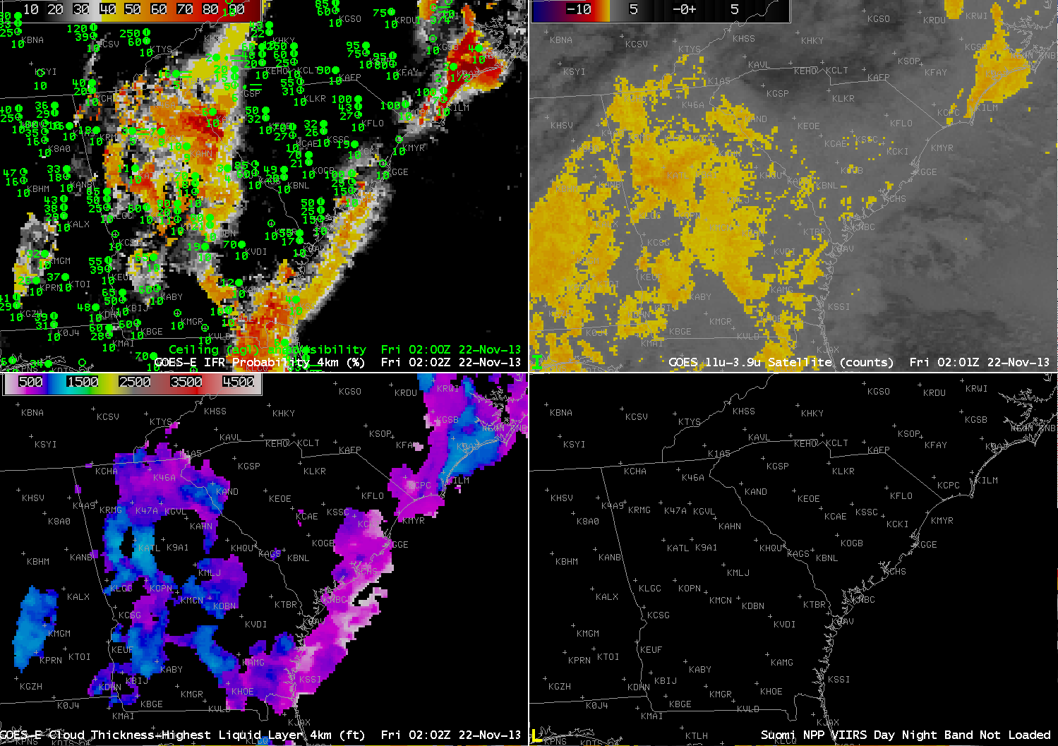
GOES-R IFR Probabilities from GOES-13 (Upper Left), GOES-13 Brightness Temperature Difference Product (10.7 µm – 3.9 µm) (Upper Right), GOES-R Cloud Thickness from GOES-13 (Lower Left), Suomi/NPP Day/Night Band (Lower Right), at 0202 UTC 22 November 2013 (click image to enlarge)

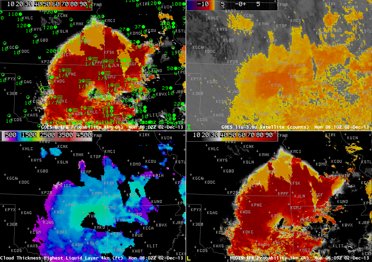
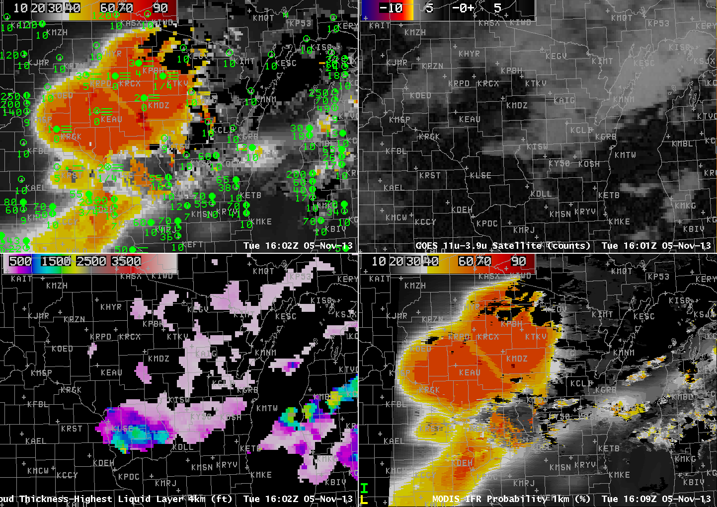
At 0315 UTC, IFR Probabilities continue to increase along the South Carolina coast. In contrast, Brightness Temperature difference fields are showing less of a signal suggestive of fog and low stratus. There was a Terra overpass at 0316 UTC that allowed MODIS data to be used in the GOES-R IFR Probability algorithm, and that field agrees well with the GOES-based field.

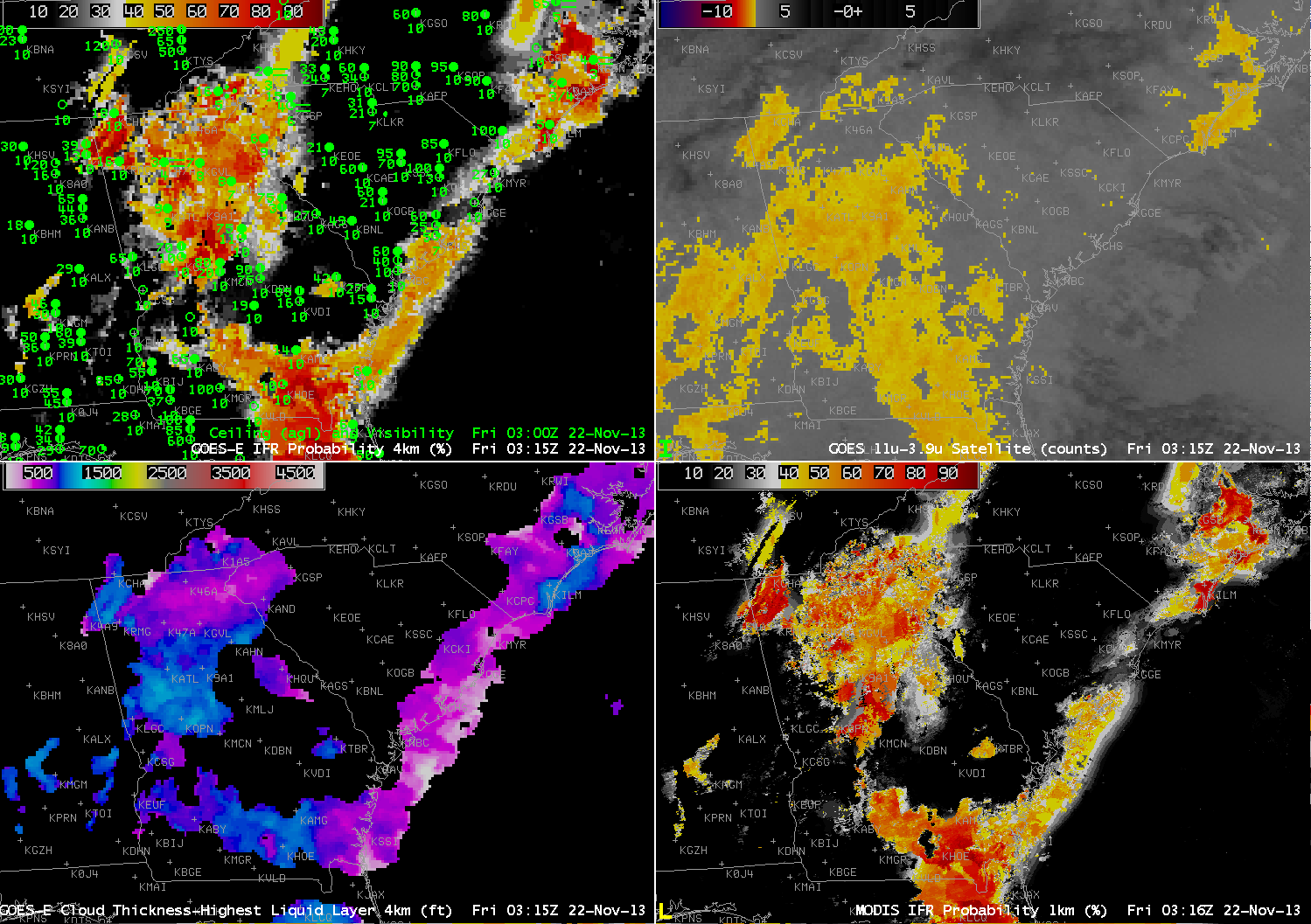
GOES-R IFR Probabilities from GOES-13 (Upper Left), GOES-13 Brightness Temperature Difference Product (10.7 µm – 3.9 µm) (Upper Right), GOES-R Cloud Thickness from GOES-13 (Lower Left), GOES-R IFR Probabilities computed from MODIS data (Lower Right), at ~0315 UTC 22 November 2013 (click image to enlarge)

At 0502 UTC, GOES-R IFR Probabilities are still high in a narrow corridor along the coast, despite the lack of a distinct signal from GOES-East in the brightness temperature difference field.

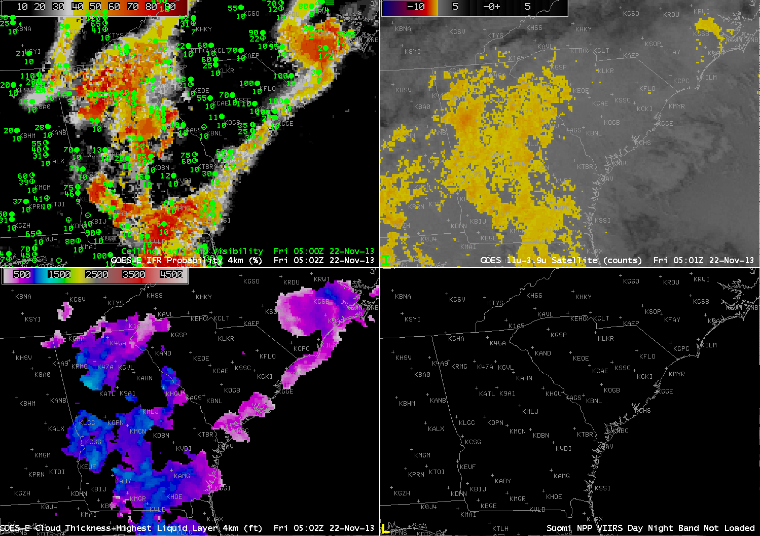
GOES-R IFR Probabilities from GOES-13 (Upper Left), GOES-13 Brightness Temperature Difference Product (10.7 µm – 3.9 µm) (Upper Right), GOES-R Cloud Thickness from GOES-13 (Lower Left), Suomi/NPP Day/Night Band (Lower Right), at 0502 UTC 22 November 2013 (click image to enlarge)

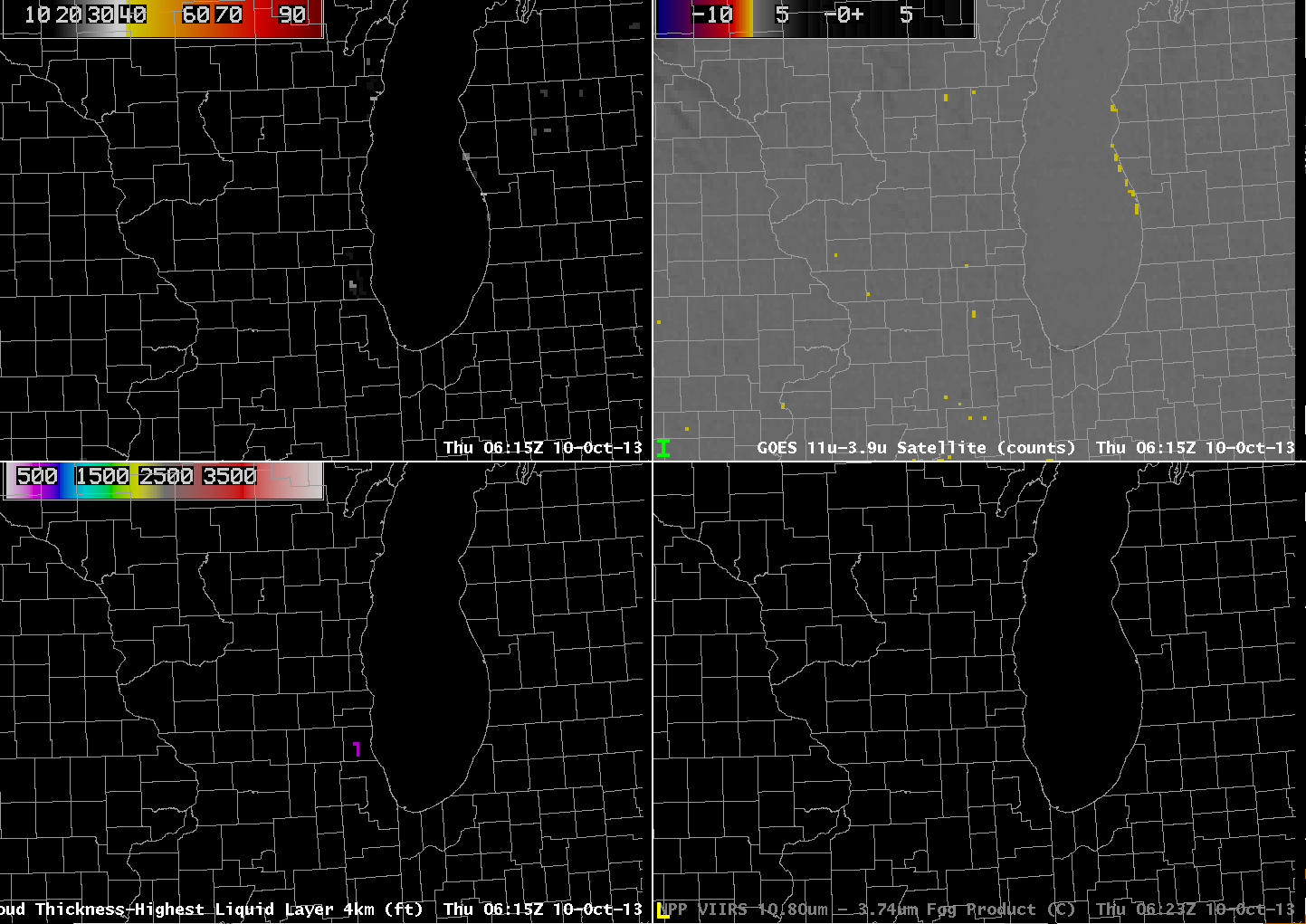
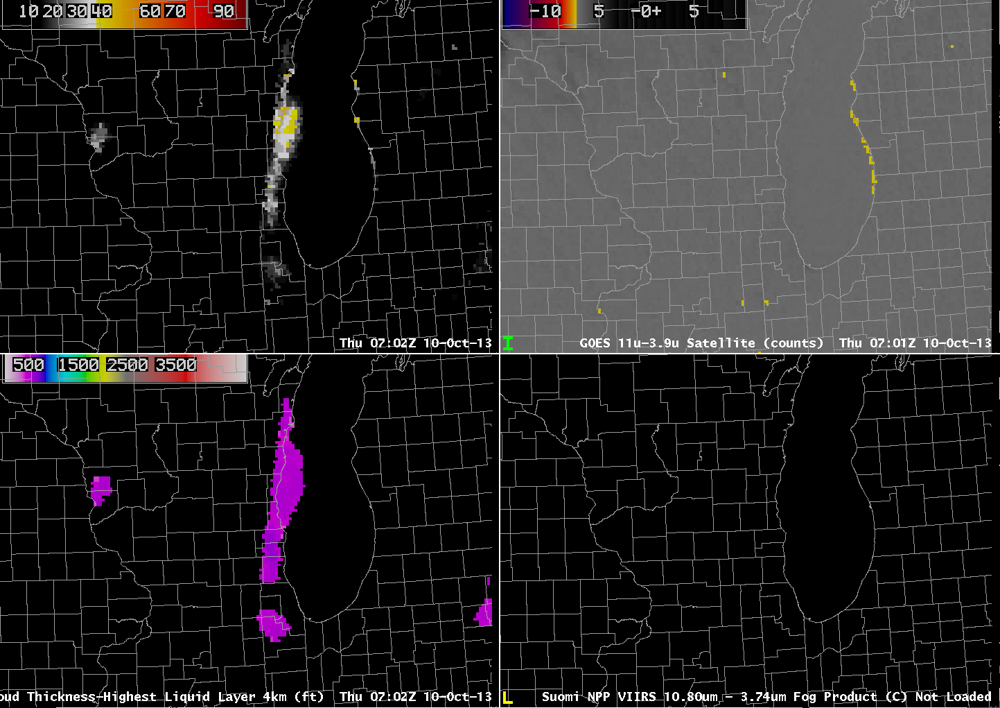
At 0615 UTC, the brightness temperature difference field starts to show a signal that is consistent with the presence of fog and low stratus along coastal South Carolina. GOES-R IFR Probabilities increase, as well. This is to be expected because the GOES-R algorithms use signals from both the GOES Satellite and the Rapid Refresh data to compute IFR Probabilities. Given that the Rapid Refresh data has been suggesting Fog/Low Stratus might be present (something that can be assumed to be true given the elevated probabilities that could alert any forecaster to the presence of developing fog that have been present for hours in the absence of a distinct signal from satellite), the appearance of a definitive satellite signal should only increase the probability of IFR conditions. At 0616, Suomi/NPP was viewing coastal South Carolina, and both the Day/Night band and the brightness temperature field are shown in the figure below. GOES-R IFR Probability algorithms do not yet incorporate Suomi/NPP data.

GOES-R IFR Probabilities from GOES-13 (Upper Left), GOES-13 Brightness Temperature Difference Product (10.7 µm – 3.9 µm) (Upper Right), GOES-R Cloud Thickness from GOES-13 (Lower Left), Toggle between Suomi/NPP Day/Night Band and Brightness Temperature Difference (Lower Right), at ~0615 UTC 22 November 2013 (click image to enlarge)

By 0800 UTC, below, IFR Conditions are reported at Charleston, SC, and GOES-R IFR Probabilities, brightness temperature difference field from GOES and Suomi/NPP and the Day/Night Band from Suomi/NPP all suggest the presence of fog/low stratus. To the northwest, over southeastern Tennessee, high clouds are obscuring the satellite view of any stratus/fog that is present (IFR Conditions are reported at, for example, Crossville, TN).

GOES-R IFR Probabilities from GOES-13 (Upper Left), GOES-13 Brightness Temperature Difference Product (10.7 µm – 3.9 µm) (Upper Right), GOES-R Cloud Thickness from GOES-13 (Lower Left), Toggle between Suomi/NPP Day/Night Band and Brightness Temperature Difference (Lower Right), at ~0800 UTC 22 November 2013 (click image to enlarge)

At 1145 UTC, IFR Probabilities maintain their high values along coastal South Carolina (and all of southwest Georgia) where IFR conditions are occurring. Note how the GOES-13 Brightness temperature difference product has highlighted values over central South Carolina, where IFR conditions are not reported. In this region, the Rapid Refresh model data is not showing saturation (or near-saturation) consistent with low-level stratus/fog so IFR Probabilities are reduced.

1145 UTC is the last image for GOES-R Cloud Thickness prior to twilight conditions. Data in the image can be used (in concert with this chart) to predict the dissipation time for radiation fog. GOES-R Cloud Thickness values over southeast Georgia range from 950 to 1100 feet, suggesting a dissipation time of 3 hours, or near 1445 UTC.

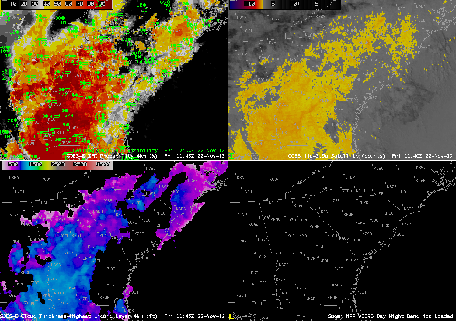
GOES-R IFR Probabilities from GOES-13 (Upper Left), GOES-13 Brightness Temperature Difference Product (10.7 µm – 3.9 µm) (Upper Right), GOES-R Cloud Thickness from GOES-13 (Lower Left), Suomi/NPP Day/Night Band (Lower Right), at 1145 UTC 22 November 2013 (click image to enlarge)

(Added: Later in the day)

Higher clouds allowed the low clouds to linger. By 1732 UTC, the low clouds had almost dissipated.

GOES-13 Visible Imagery, 1732 UTC 22 November 2013 (click image to enlarge)

Fog/Low Stratus over southwest Alaska on November 8

GOES-15-based GOES-R IFR Probabilities every half hour from 0300 UTC through 1530 UTC (click image to animate)

Fog and low stratus were present over southwestern Alaska early on November 8. How did the GOES-R IFR Probability fields perform compared to the heritage brightness temperature difference (in this case, 10.7 µm – 3.9 µm from GOES-15). Consider the airport PARS (southwest of Anvik — PANV and northwest of Aniak — PANI). IFR conditions are present there until 0900 UTC, when ceilings rise and IFR probabilities drop. Subsequently, IFR Probabilities increase again as a north-south oriented region of higher IFR probabilities moves over, and IFR conditions are again present by 1600 UTC. Further south, PAJZ and PAIG report IFR conditions when IFR Probabilities are high, and conditions improve as IFR Probabilities decrease. IFR Probabilities initially around PAIG have the characteristic flat field (and somewhat lower probability) associated with a region where high-level clouds are present. In these regions, only Rapid Refresh data can be used to compute the probability; because satellite predictors are not used, the computed IFR probabilities are lower.

Compare the IFR Probability field, above, to the Brightness Temperature Difference field, below, that has been color-enhanced to highlight regions where water-based clouds may be present. The IFR Probability field correctly reduces the regions where IFR conditions might be occurring. That is, the traditional brightness temperature difference field is plagued by many false positives. This is because mid-level stratus that is unimportant for transportation looks to a satellite to be very similar to low-level stratus that is important for transportation.

GOES-15 Brightness Temperature Difference (10.7 µm – 3.9 µm) every hour from 0300 UTC through 1500 UTC (click image to animate)

MODIS data from the polar-orbiting satellites Terra and Aqua can also be used to compute IFR Probabilities, and MODIS data — although less frequent than the data from the geostationary GOES-15 — has far superior horizontal resolution (nominal MODIS resolution is 1 km at nadir) to GOES data (nominally 4 km at the sub-satellite point over the Equator) over Alaska. Small-scale features are much more likely to be detected in MODIS data, as shown below.

GOES-15-based GOES-R IFR Probabilities (Upper Left), GOES-15 Brightness Temperature Difference Product (10.7 µm – 3.9 µm) (Upper Right), Suomi-NPP Brightness Temperature Difference (11.45 µm – 3.74 µm) and Day/Night band (Lower Left), MODIS-based GOES-R IFR Probabilities (Lower Right), all times as indicated (click image to enlarge)

The Day/Night band from Suomi/NPP can sometimes be used to detect cloud features. However, when the Moon is not present to provide illumination, cloud detection is a challenge. In the toggle above between the Day/Night band and the brightness temperature difference from VIIRS (11.45 – 3.74), for example, there is little evidence of the apparent cloud edge that is visible both in VIIRS data, in GOES-15 data (Upper right) and in the IFR Probability fields from GOES (Upper Left) and MODIS (Lower Right).

Fog and Stratus in one scene: What should be highlighted?

GOES-13-based GOES-R IFR Probabilities (Upper Left), GOES-13 Brightness Temperature Difference Product (10.7 µm – 3.9 µm) (Upper Right), GOES-R Cloud Thickness (Lower Left), Suomi-NPP Day/Night band (Lower Right), all times as indicated (click image to enlarge)

Dense fog developed over Western Wisconsin before sunrise on 5 November 2013. The animation above shows the development of high IFR probabilities in that region as a mid-level stratus deck shifts off to the east. Cloud thicknesses just before sunrise reach 1100 feet over portions of Wisconsin; according to this plot, fog should persist for at least 4 hours after sunrise. This was the case. Fog dissipated shortly after 1700 UTC.

This case shows a benefit of the GOES-R IFR Probability field: it accurately discerns the difference between low stratus/fog (that develops over western Wisconsin) and mid-level stratus (retreating to the east over central and eastern Wisconsin during the animation). Mid-level stratus is normally not a transportation concern whereas low clouds/fog most definitely are; in this case, dense fog advisories were issued by the Lacrosse, WI, WFO (ARX). At the beginning of the animation, widespread mid-level stratus is indicated (IFR conditions are not reported). As the night progresses, IFR Probabilities increase in regions where IFR conditions start to be reported. (A brightness temperature signal in GOES also develops in this region).

As above, but at 0815 UTC. The lower right image toggles between the Day/Night Band and the Brightness Temperature Difference (11.45 µm – 3.74 µm) from Suomi/NPP (click image to enlarge)

Suomi/NPP VIIRS viewed this scene shortly after 0815 UTC, and that imagery is above. Both the Day/Night band and the Brightness Temperature Difference fields (11.45 µm – 3.74 µm) are shown as a toggle. The mid-level stratus at 0815 is readily apparent. The developing fog over river valleys in western Wisconsin shows plainly in the brightness temperature difference field, but less so in the day/night band with scant lunar illumination.

GOES-13-based GOES-R IFR Probabilities (Upper Left), GOES-13 Brightness Temperature Difference Product (10.7 µm – 3.9 µm) (Upper Right), GOES-R Cloud Thickness (Lower Left), MODIS-based IFR Probabilities (Lower Right), all times as indicated (click image to animate)

MODIS data from Terra and Aqua is also used to produce IFR Probabilities, and those data are shown above, for three times: 0413 UTC, 0823 UTC and 1609 UTC. Patterns in the MODIS IFR Probability are similar to those in GOES, but small-scale features such as river valleys are much more apparent. Note that by 1609 UTC, higher clouds have overspread western Wisconsin in advance of an approaching mid-latitude cyclone; thus, the GOES and MODIS IFR Probabilities both are flat fields that are mostly based on Rapid Refresh data. Nevertheless, they both depict the region of IFR conditions over western Wisconsin that is surrounded by better visibilities and higher ceilings. Recall that GOES-R cloud thickness is not computed where high clouds are present.

Fog and Stratus under high clouds in the Southern Plains

GOES-13-based GOES-R IFR Probabilities (Upper Left), GOES-13 Brightness Temperature Difference Product (10.7 µm – 3.9 µm) (Upper Right), MODIS-based GOES-R IFR Probabilities (Lower Left), Suomi-NPP Brightness Temperature Difference (11.35 µm – 3.74 µm) and Day/Night band (Lower Right), all times as indicated (click image to enlarge)

Fog and low stratus developed over the Southern Plains during the morning hours of 28 October 2013. The imagery above, from near 0730 UTC, demonstrates strengths of the IFR Probability fields and inherent limitations to the traditional methods of detecting fog and low stratus: the brightness temperature difference between 10.7 µm and 3.9 µm data. For example, note the elevated stratus over the Red River Valley in southeastern OK. Both GOES and VIIRS Brightness Temperature Difference fields there show a strong signal (and the day/night band also suggest clouds are present); IFR Probabilities are low, however, and are in good agreement with the observed ceilings and visibilities that show MVFR conditions.

The brightness temperature difference fields from both Suomi/NPP and from GOES show high clouds over south-central OK, in a region where IFR Conditions are observed. Rapid Refresh model data are being used in this region to diagnose — accurately — the presence of visibility-restricting fog and low stratus. As is typical when Rapid Refresh data are the primary means of diagnosing IFR Probabilities (because high clouds prevent the satellite from seeing water-based clouds near the surface), the IFR probability field is smooth.

IFR Conditions in the northern Plains

GOES-13-based GOES-R IFR Probabilities (Upper Left), GOES-13 Brightness Temperature Difference Product (10.7 µm – 3.9 µm) (Upper Right), MODIS-based GOES-R IFR Probabilities (Lower Left), Suomi-NPP Brightness Temperature Difference (11.35 µm – 3.74 µm) (Lower Right), all times as indicated (click image to enlarge)

The animation above shows GOES-R IFR Probabilities highest in a band that stretches mostly north-south from western North Dakota into central South Dakota. IFR conditions are observed under and near this band, for example at Stanley, North Dakota. The occasional MODIS-based IFR Probabilities also suggest that IFR conditions are most likely over the western Dakotas. Both GOES-based and MODIS-based IFR Probability fields de-emphasize the regions of enhanced brightness temperature difference (in both GOES and Suomi-NPP Fields) that exist over western Minnesota and the central and eastern Dakotas. In these regions, mid-level stratus is being detected by the satellite. The Rapid Refresh model is correctly diagnosing the clouds as elevated, and that model information is used to de-emphasize (correctly) the possibility of IFR conditions. IFR and near-IFR conditions also occur over parts of northeast Minnesota into northwest Wisconsin where IFR probabilities are higher.

Toggle between GOES-13-based GOES-R IFR Probabilities and GOES-13 Brightness Temperature Difference (10.7 µm – 3.9 µm) at 0945 UTC on 22 October (click image to enlarge)

A limitation of the traditional brightness temperature difference product is highlighted above in the toggle between the GOES-R IFR Probability and the Brightness Temperature Difference at 0945 UTC. Mid-level stratus and low stratus/fog look nearly identical in the brightness temperature difference product, but the latter is very significant for aviation. Thus the need to better highlight regions of IFR conditions by using the fused data product that incorporates surface information by way of the Rapid Refresh model.

Lunar illumination is particularly strong at this time (Full moon occurred late last week), so the day/night band on Suomi/NPP gives compelling visible imagery. As with the case with brightness temperature difference products, however, it can be difficult to distinguish between mid-level stratus and low stratus in the Day/Night band. Toggles between the Day/Night band and the Brightness Temperature Difference from Suomi/NPP is at both 0736 and 0918 UTC are below. Work proceeds on incorporating Suomi/NPP data into the GOES-R IFR Probability algorithm.

Fog around Puget Sound

GOES-15-based GOES-R IFR Probabilities (Upper Left), GOES-15 Brightness Temperature Difference Product (10.7 µm – 3.9 µm) (Lower Left), MODIS-based GOES-R IFR Probabilities (Upper Right), Suomi-NPP Day/Night Band (Lower Right), all times as indicated (click image to enlarge)

IFR Conditions developed around the Puget Sound during the night of 20 October. How did the GOES-R IFR Probabilities capture this event? The animation above includes imagery from 0500, 0900, 0945, 1115 and 1915 UTC. Higher-resolution polar orbiter data (from MODIS and Suomi/NPP) shows the value of higher-resolution in capturing fog that settles into valleys over southeast British Columbia and western Washington. GOES data are unable to resolve those features.

The Brightness Temperature difference fields have a strong signal over the Pacific Ocean and adjacent coastal areas (IFR Probabilities are high in those regions: both satellite data and Rapid Refresh data are consistent with a high likelihood of fog/low stratus). Over land, the signal is more noisy, perhaps because of differences in land emissivity. (That noise is not present when the sun is up — at that time the brightness temperature difference signal is determined by reflected solar radiation). Where the brightness temperature difference signal is smaller over land, the IFR Probability is also lower. That it is not even smaller suggests that model fields are at or near saturation over land. Note also a strength of the IFR Probability: A consistent signal both day and night. IFR Probabilities are high over Seattle where IFR conditions persist.

As above, but for times with Day/Night band data at night only (click image to enlarge)

The Suomi-NPP Day/Night band can give a good indication of where clouds are present at night when, as occurred last night, the moon is near full. (The Day/Night band does not, however, by itself give any indication of surface visibility) In the example above, the clouds do not change much in the 90 minutes between overpasses. (The slight shift in the apparent location of snow-covered mountains is apparently due to parallax) GOES can just barely resolve the very thin fog features that are so evident in the Suomi/NPP data.

Fog Development near Lake Michigan

GOES-13-based GOES-R IFR Probabilities (Upper Left), GOES-13 Brightness Temperature Difference Product (10.7 µm – 3.9 µm) (Upper Right), GOES-13-based GOES-R Cloud Thickness (Lower Left), Suomi/NPP Brightness Temperature Difference (Lower Right), all near 0615 UTC on 10 October (click image to enlarge)

The GOES-R IFR Probability product gave useful advance warning to the development of fog near Lake Michigan’s eastern shore overnight. The image above, from 0615 UTC, shows a flat brightness temperature difference field over the lakeshore counties in Wisconsin and Illinois (values are from -7.1 to -7.3); there are two regions of high values in the IFR Probability field, however: Near Manitowoc WI (values up to 29%) and over southeast WI and northeast IL (values near 20%). So by 0615 UTC on 10 October, IFR Probabilities are suggestive of a nascent fog development.

As above, but for 0702 UTC on 10 October (click image to enlarge)

Forty-five minutes later, at 0702 UTC (above), IFR Probabilities have increased dramatically in eastern WI even as the brightness temperature difference field remains flat. Thus, the Rapid Refresh Data is accurately capturing the development of low-level saturation in the atmosphere, and that is influencing the IFR probability field. In addition, the GOES-R Cloud Thickness field is suggesting that the cloud bank is 500-600 feet thick. The strip of enhanced brightness temperature difference paralleling the Lake Michigan shore in lower Michigan is an artifact of the co-registration error between the 10.7 µm and 3.9 µm band detectors on GOES-13. Between 0656 UTC and 0734 UTC, visibility at Manitowoc, WI (KMTW), dropped from 5 to 3/4 statute miles. The visibility at Burlington WI (KBUU) dropped from 4 to 1 statute miles between 0600 and 0700 UTC, and Waukegan, IL (KUGN) reported a visibility of 1/4 mile at 0552 UTC and 0652 UTC.

As above, but for 0802 UTC on 10 October (click image to enlarge)

At 0802 UTC, the GOES-East brightness temperature difference field shows greater differences over the region of SE Wisconsin where the fog is developing. Accordingly, the IFR probability increases past 80% IFR Probabilities are near 70% in Manitowoc County (and Manitowoc reported 1/2-mile visibility at 0834 UTC). Compare the GOES-East and Suomi/NPP Brightness Temperature Difference Fields; note the lack of a signal in the Suomi/NPP field along the western shore of Lake Michigan, confirming the co-registration error present in GOES-13.

As above, but for 1145 UTC on 10 October (click image to enlarge)

The last pre-sunrise image, 1145 UTC, shows a definite signal of fog/low stratus in both the IFR Probability field and in the Brightness Temperature Difference field. However, the early detection in the IFR Probability field gives a nice head’s up to the forecaster. Note also in this image how the strong signal in the brightness temperature difference field that arises because of the co-registration error can contaminate the IFR Probability field. The Cloud Thickness in this field has been related to dissipation time, as shown in this chart. The maximum thickness of 1000 feet predicts a dissipation time around 1500 UTC. The 1445 and 1515 UTC GOES-13 visible images are shown below.

GOES-13 Visible Imagery at 1445 UTC and 1515 UTC on 10 October (click image to enlarge)

GOES-R Fog Product Examples

Fog detection fusing GOES, Terra/Aqua or Suomi/NPP Satellite data with Model output