Category Archives: Suomi/NPP

Fog over Pennsylvania

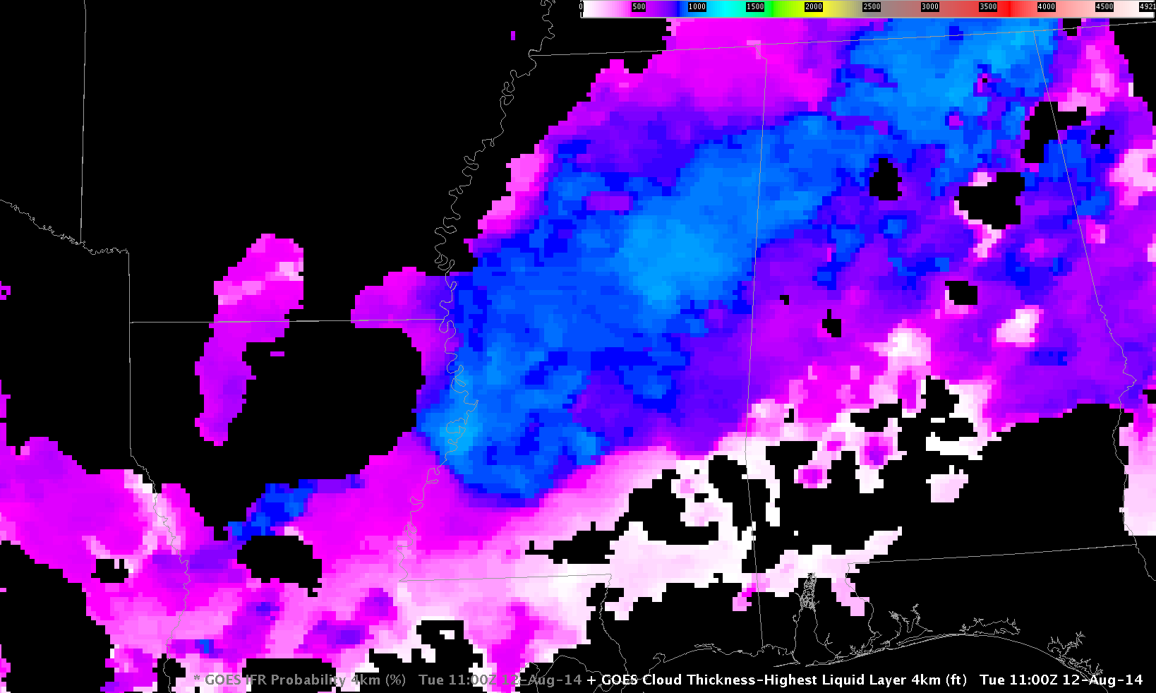
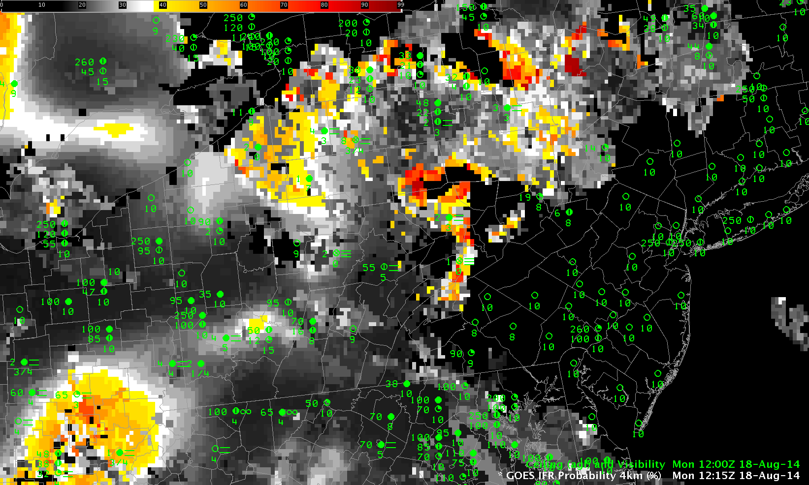
GOES-R IFR Probabilities computed from GOES-13 data, hourly from 0500 through 1300 UTC 18 August 2014

River valley fog developed over Pennsylvania during the early morning hours of 18 August 2014, and the case is a good test of the GOES-R IFR Probability fields. IFR Probabilities are low at 0500 UTC (1 AM local time) and subsequently increase rapidly. In this case, the fields may be overpredicting where fog is present, as visible imagery just after sunrise suggest it was confined mostly to river valleys. In the animation above, the areal extent of the IFR Probabilities drops between 1100 UTC and 1215 UTC as the sun rises (the terminator is apparent in the 1100 UTC image, running from western Maryland north-northwestward to extreme western New York) and visible imagery can be used to more effectively cloud-clear the fields. A toggle between these two times is below. In this case, it is important to understand the geography underneath the IFR Probability field to hone the forecast.

GOES-R IFR Probabilities computed from GOES-13 data, at 1100 and 1215 UTC 18 August 2014

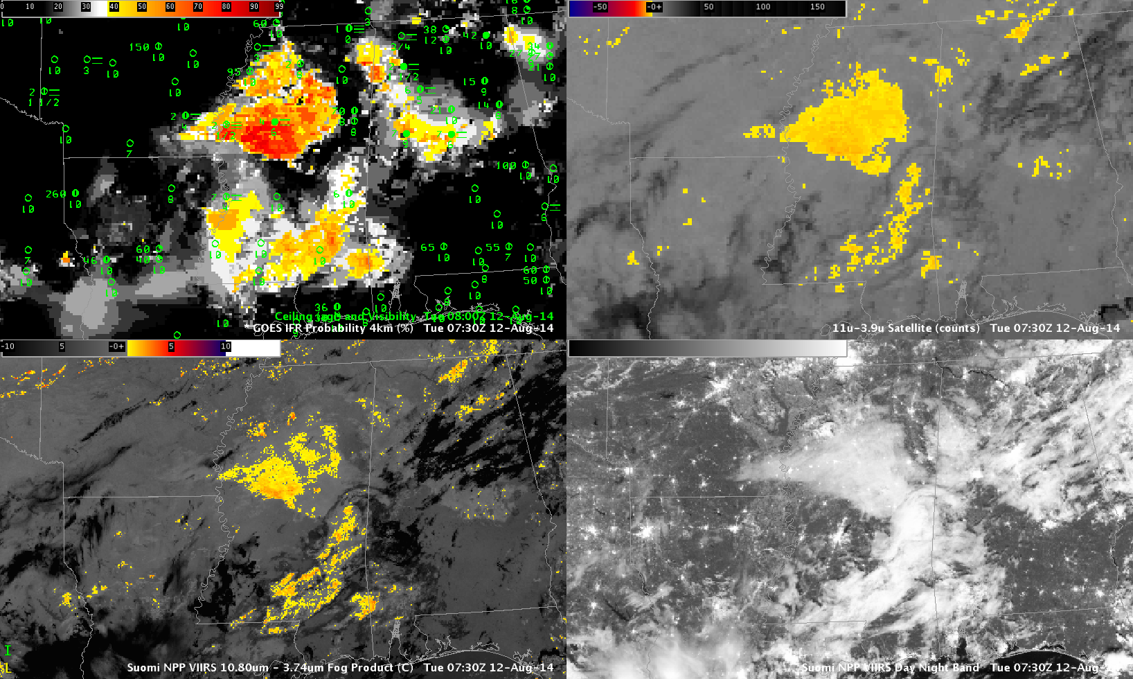
GOES-East Brightness Temperature Difference Fields (10.7µm – 3.9µm), hourly, from 0500-1100 UTC 18 August 2014

The Brightness Temperature Difference field, above, is the heritage method of detecting low stratus and inferring the presence of fog. Interpretation is complicated because high clouds (initially present over the southwestern portion of the scene, and moving eastward) prevent the satellite from viewing low clouds. In addition, as the sun rises (at the end of the animation, at 1100 UTC), solar radiation changes the character of the the brightness temperature difference field.

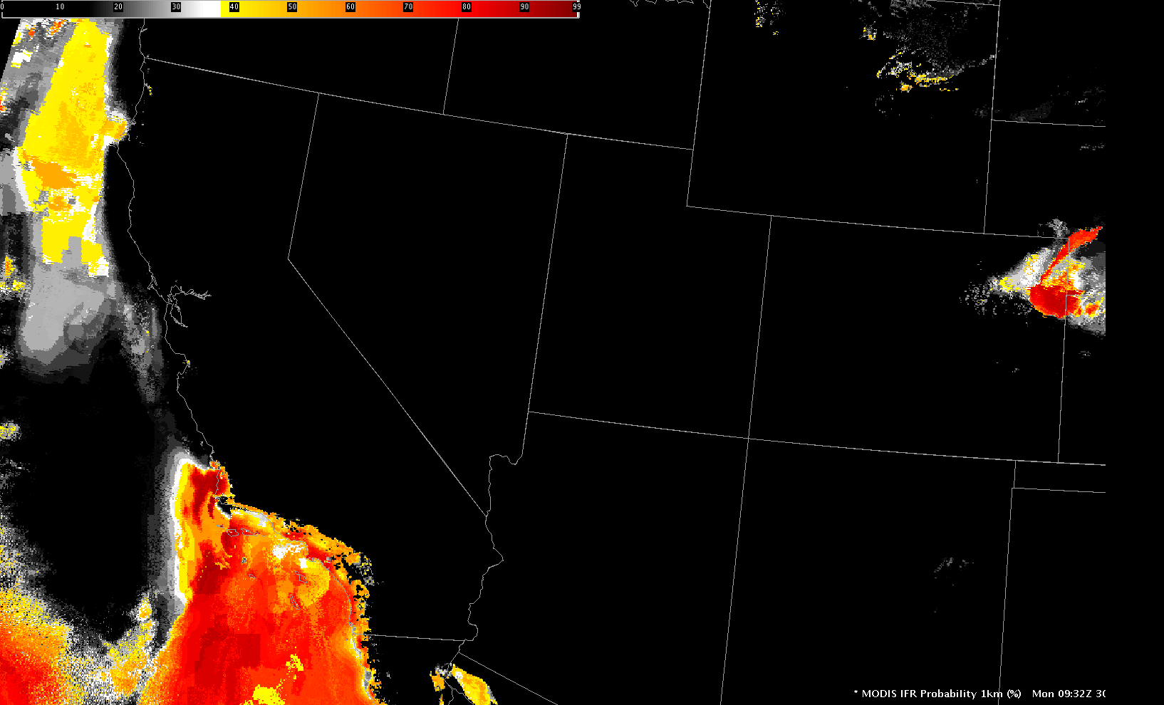
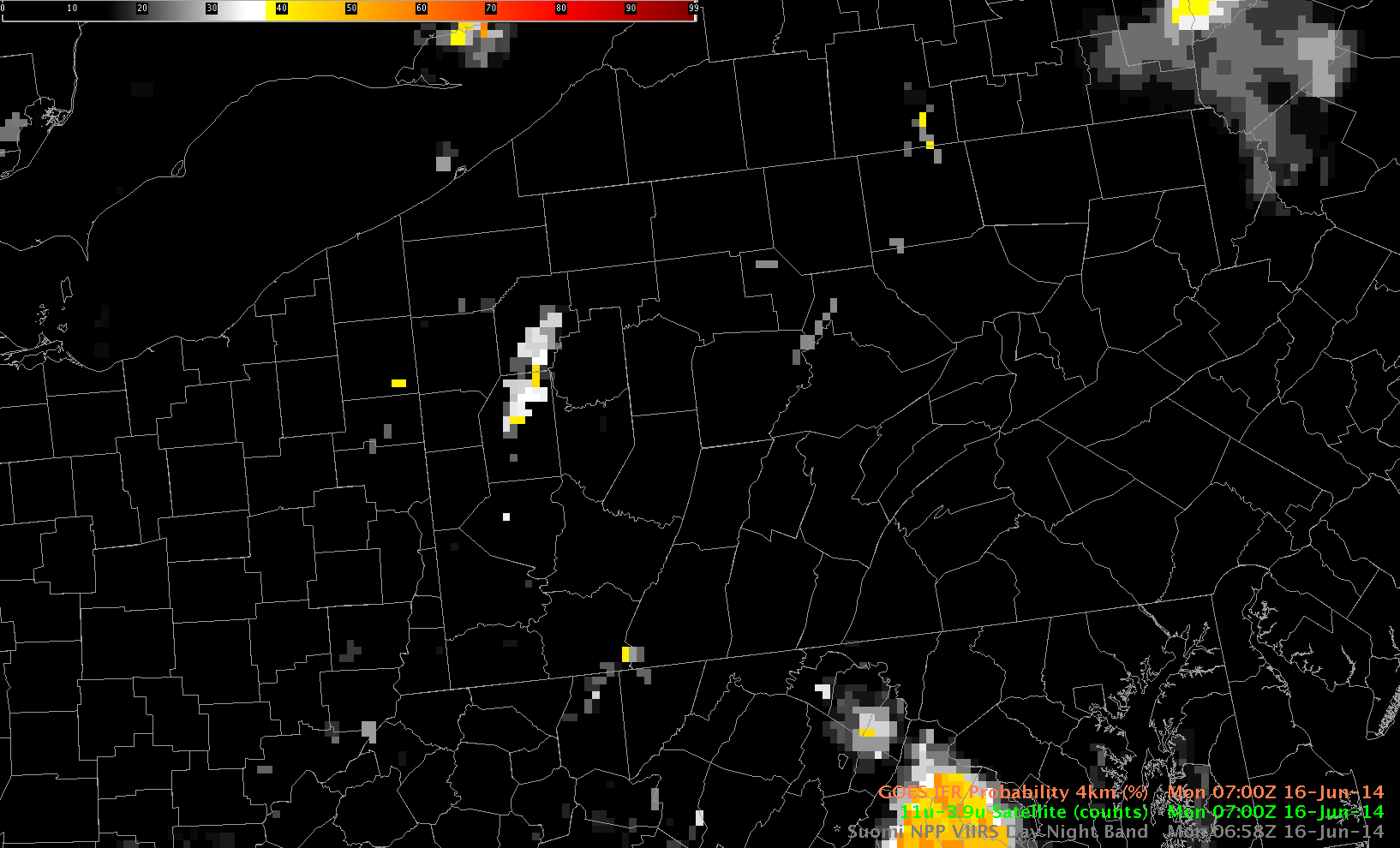
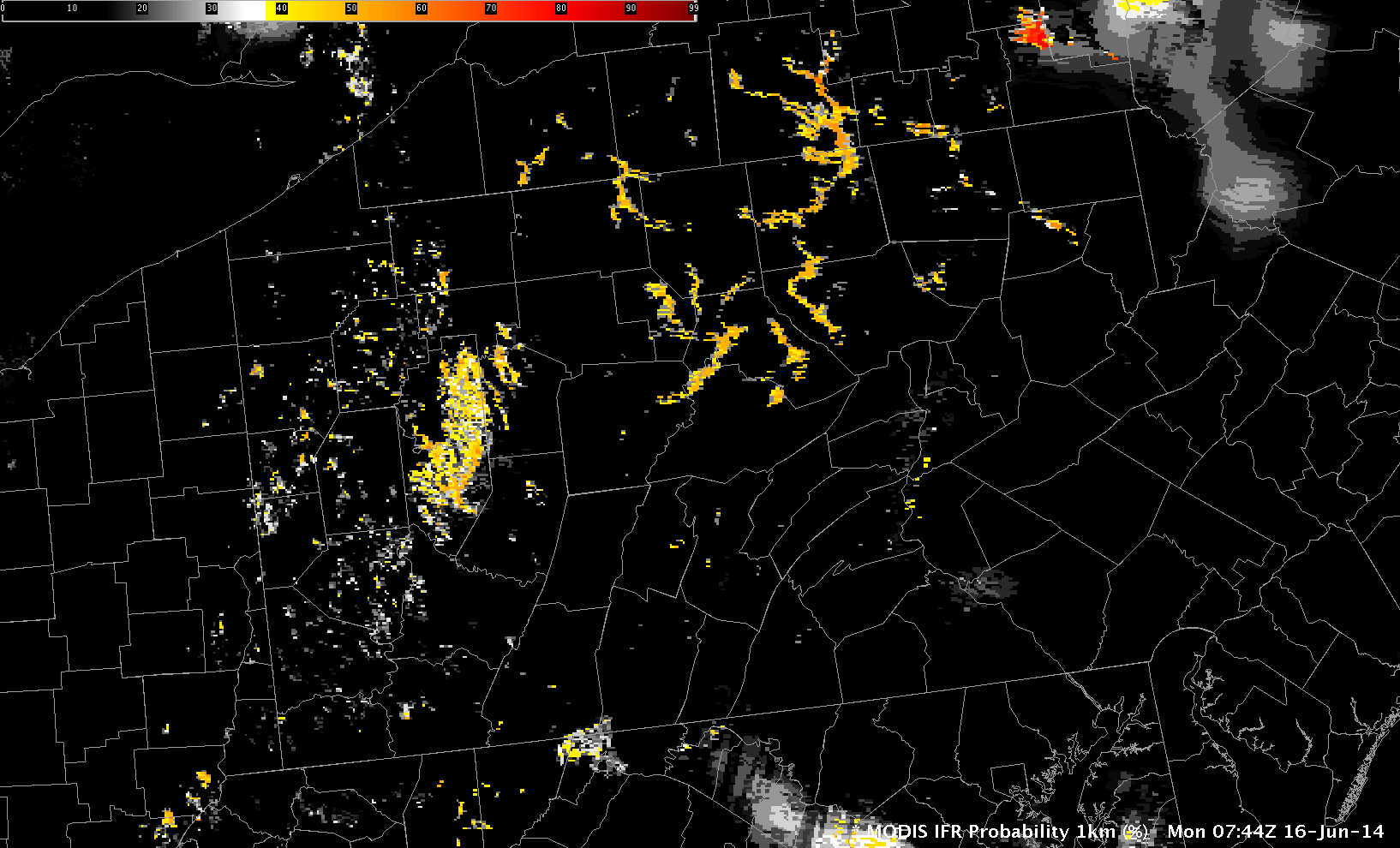
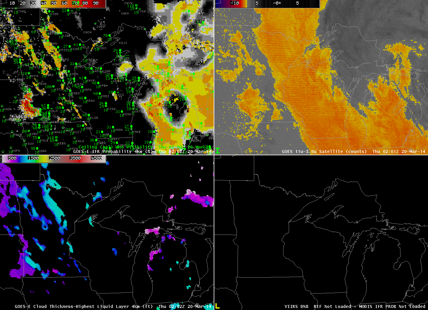
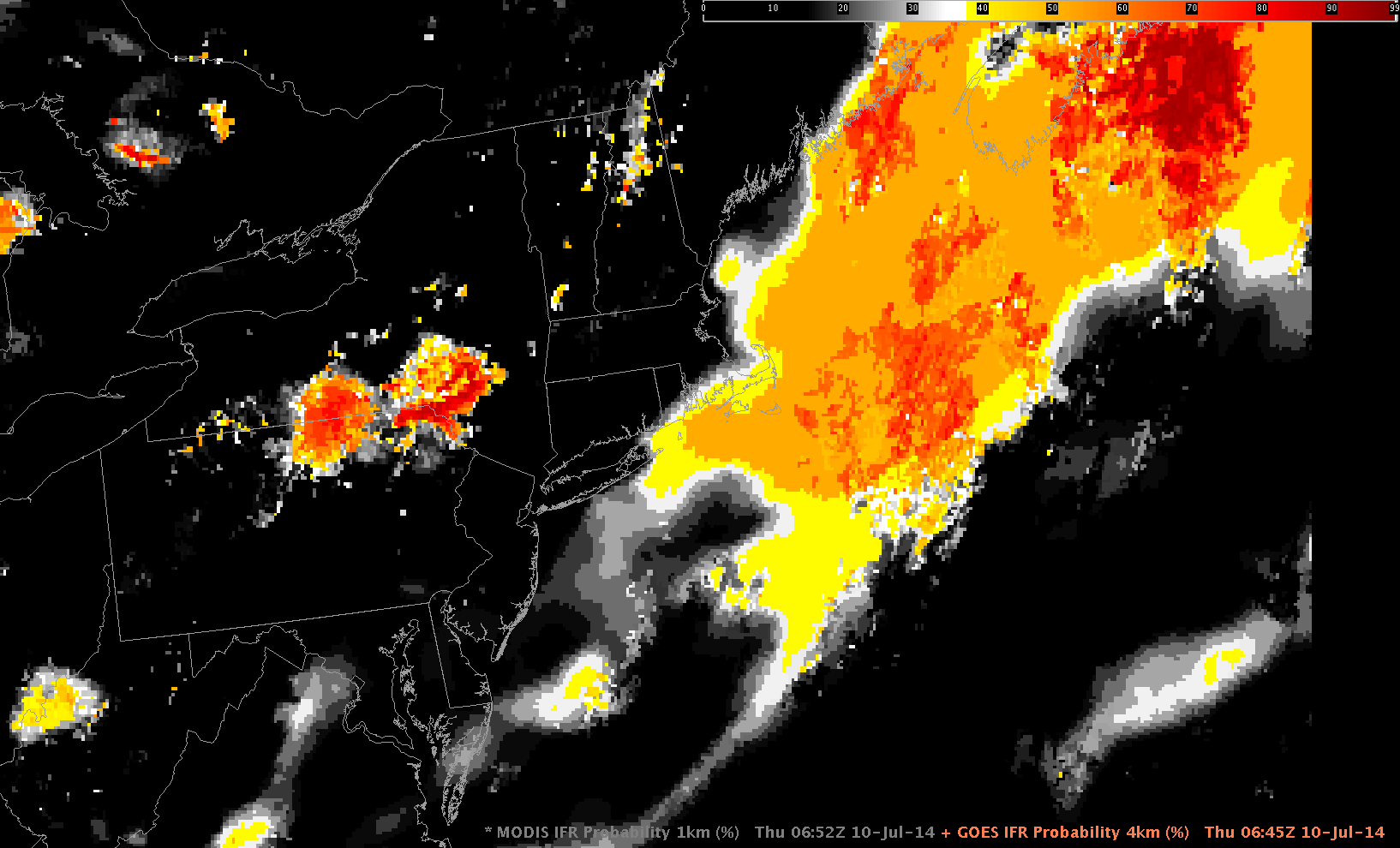
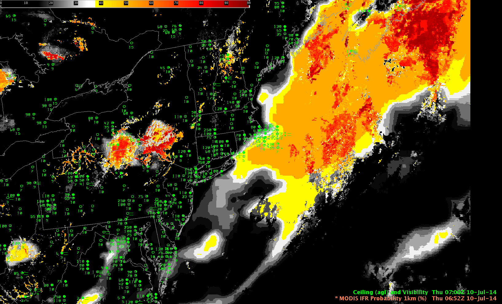
Data from the MODIS on board both Terra and Aqua can also be used to create both brightness temperature difference fields and IFR Probability fields. The toggle below, using ~0700 UTC data from GOES and from MODIS, shows the distinct advantage present in the MODIS field’s superior spatial resolution (1-km at sub-satellite point vs. 4-km at the sub-satellite point for GOES). River valleys are more evident in the MODIS data, by far, than in the GOES data.

GOES-R IFR Probabilities computed from GOES-13 data and from MODIS data, at 0700 UTC 18 August 2014

The Day-Night band on Suomi NPP at 0718 UTC showed that the densest fog was largely confined to river valleys.

Suomi NPP Day/Night Band, 0718 UTC on 18 August 2014

An animation of the fog burning off from GOES-14 (in special 1-minute SRSO-R scanning operations) is available here. It’s also on YouTube.

Fog over Mississippi

GOES-R IFR Probabilities computed from GOES-13 at 0730 UTC (Upper Left), GOES-13 Brightness Temperature DIfference (10.7 µm – 3.9 µm) (Upper Right), Suomi NPP VIIRS Brightness Temperature Difference (11.35 µm – 3.74 µm) (Lower Left), Suomi NPP VIIRS Day Night Band (Lower Right), all at 0730 UTC on 12 August 2014

Fog developed overnight in central Mississippi, and the imagery above, at 0730 UTC, is a snapshot during the development. The just-past-full moon provided plenty of illumination, so the stratus and cirrus clouds over the south are distinct. It can be difficult, however, using only the Day Night Band to distinguish between low stratus (north-central Mississippi), mid-level stratus (eastern Mississippi), and high, thick cirrus (Alabama). In addition, the Day Night Band and the brightness temperature difference fields give information at the top of the cloud only. Information about the bottom of the cloud — whether the stratus deck extends to the surface as fog, for example, is difficult to glean from cloud-top properties. This is where the IFR Probability field that incorporates both cloud-top features derived from the brightness temperature difference field and lower-tropospheric information extracted from the Rapid Refresh Model can improve the detection of reduced ceilings and visibilities. Suomi NPP and other polar orbiters can give high spatial resolution imagery. GOES data has excellent temporal resolution to monitor how things evolve with time. The animation below shows how the fog/low stratus developed over the course of the day.

GOES-R IFR Probabilities and Surface observations of visibility/ceilings, hourly 0200-1100 UTC 12 August 2014

The fields in the animation above change character over the course of the night. Initially, the fields over southwestern Mississippi are very smooth; in this region, multiple cloud layers (a thunderstorm complex was dissipating) prevent any satellite signal from being used as a predictor for IFR Probabilities; only model data are being used. As the night progresses and the mid-level and upper-level clouds dissipate, the character of the field takes on a more pixelated appearance that means satellite data are being used as a predictor. The addition of satellite data to the suite of predictors also means that the probability value increases. By the end of the night, high probabilities have overspread much of central Mississippi, and low ceilings and reduced visibilities are widespread.

GOES-R Cloud Thickness can be used to estimate times of fog dissipation, using the relationship in this scatterplot and the Cloud Thickness in the last pre-sunrise scene, shown below for 12 August 2014. The thickest values are near Vicksburg, MS, where GOES-R Cloud Thickness approaches 1000 feet. That suggests a clearing time around 1400 UTC, ~3 hours after the valid time of the image below. The visible animation of the low clouds clearing is below.

GOES-R Cloud Thickness, 1100 UTC 12 August 2014

Fog in the Ohio Valley

GOES_OBS_BTD_SNPPBTD_MODISIFR_04August2014_0815

GOES-R IFR Probabilities and Surface observations of Ceiling and Visibility (Upper Left), GOES-East Brightness Temperature Difference (10.7 µm – 3.9 µm) (Upper Right), Suomi-NPP Brightness Temperature Difference (11.35 µm – 3.74 µm) (Lower Left), MODIS-based IFR Probabilities and Brightness Temperature Difference (11.0 µm – 3.9 µm) (Lower Right), all times as indicated

There are different ways to alert a forecaster to the presence of a transporation hazard like low ceilings and reduced visibilities. The imagery above shows GOES-based (nominal 4-km resolution at nadir) products (top) and Suomi/NPP and MODIS-based products (nominal 1-km resolution — or better — at nadir). The Brightness Temperature Difference from GOES (upper right) overestimates the region with lowered ceilings; in contrast, the IFR Probability field (upper Left) is able to distinguish between elevated stratus and low stratus because it includes information from the Rapid Refresh model to identify regions with saturation in the lowest levels of the atmosphere. This allows the IFR Probability to screen out regions of mid-level stratus.

The Suomi NPP and MODIS Brightness Temperature Difference fields do not suggest widespread stratus as does the GOES-based Brightness Temperature Difference field. Rather, the data from the polar orbiters suggest regions of stratus or fog in river valleys over Kentucky, Indiana and Illinois. MODIS-based IFR Probability (Lower Right) agrees with the GOES-based IFR Probability field: a region of fog/low stratus is developing over southwestern Indiana and southeastern Illinois, near the Wabash River. In this case, the model data is helping to strengthen a weak signal in a region where fog is present. Model data is a key strength in the IFR Probability field.

Polar orbiters give excellent horizontal resolution, but only GOES provides the high temporal resolution necessary to monitor the development of fog/low stratus. The toggle between 0800 and 1100 UTC, below, for example, depicts an increase in fog. A single GOES satellite can (and does) monitor that increase. A suite of polar orbiters would be required to give similar temporal coverage in middle latitudes.

As above, times as indicated

Distinguishing between stratus and fog over Pennsylvania

Suomi NPP 11.35 µm Infrared Imagery at 0609 and 0752 UTC, 10 July 2014 (Click to enlarge)

The orbital geometry of Suomi NPP allowed two high-resolution images of Pennsyvlania early in the morning of the 10th of July 2014. Can you tell from the imagery above if there is fog/stratus in the river valleys of Pennsyvlania? Are the relatively cool clouds from Pittsburgh northeastward towards Elmira, NY obstructing visibilities? Based on the IR (11.35 µm for Suomi NPP) imagery alone, above, that is a difficult question to answer. Historically, the brightness temperature difference between the longwave IR (11.35 µm) and the shortwave IR (3.74 µm) has been used to indentify water-based clouds. Imagery from Suomi NPP, below, highlights where water-based clouds (like stratus) exist. If the clouds are the same temperature as the surrounding land (likely the case for river fog), a single 11.35-µm image is of little help in identifying the clouds.

Suomi NPP 11.35 – 3.74 µm Brightness Temperature Difference at 0609 and 0752 UTC, 10 July 2014 (Click to enlarge)

The Day-Night band can also highlight where clouds exist, because lunar illumination reflects well off clouds. A 3/4-full moon ably illuminates the scene at 0609 UTC, but that moon has set at 0747 UTC and the Clouds are harder to see.

Suomi NPP Day/Night Band at 0609 and 0752 UTC, 10 July 2014 (Click to enlarge)

Both the Day/Night band and the Brightness Temperature Difference Fields (and any Infrared image) gives information about the top of the cloud. Fog existence is difficult to discern only from satellite data because the bottom of the cloud is not sampled. This is why a fused product (such as IFR Probability) that includes surface information (in the case of IFR Probability from the Rapid Refresh Model) is desirable. MODIS data can be used to compute IFR Probability, and a MODIS-carrying Aqua pass occurred in between the two Suomi NPP Passes shown above.

MODIS 11 – 3.9 µm Brightness Temperature Difference and IFR Probability at 0652 UTC, 10 July 2014 (Click to enlarge)

In the two images above, note how the IFR Probability Fields de-emphasize the low cloud areas that stretch northeastward from Pittsburgh towards Elmira. This is likely mid-level stratus. River Fog over northeast Pennsylvania is highlighted in the IFR Probability fields (and in the brightness temperature difference field). This image, which shows the GOES-based IFR Probability field at 0645 UTC, highlights the power of MODIS’ superior spatial resolution in the early detection of small-scale fog. The large region of reduced visibility around Elmira NY (meager surface observations suggest this large region of fog verified) appears in both MODIS- and GOES-based IFR Probability fields. Only the MODIS-based IFR Probability field, however, has a distinct river-valley signal over northeast Pennsylvania.

MODIS and GOES IFR Probability both suggest IFR conditions may be occurring over the Atlantic Ocean. The brightness temperature difference field shows no low cloud signal there because of a cirrus shield. IFR Probability gives a signal of fog here based on information from the Rapid Refresh.

MODIS-based IFR Probability over California

MODIS-based IFR Probabilities over the western US, 0932 UTC on 30 June 2014 (Click to enlarge)

MODIS data, although infrequent, can give a high-resolution estimate of whether of not fog/low clouds are forming in a region. This is particularly useful for cases with highly variable terrain (such as deep river valleys). In the image above, IFR Probabilities are very low over both the Central Valley of California and over the Salinas Valley closer to the coast. Fog/low Stratus are unlikely to be occurring.

Suomi/NPP Brightness Temperature Difference Fields (11.35µm – 3.74µm) at 0916 and 1057 UTC on 30 June 2014 (Click to enlarge)

The orbital geometry of Suomi/NPP on June 30th was such that it provided two close-up views of these two valleys around/after the time of the MODIS pass shown above. The animation above toggles between those two times. The brightness temperature difference field shows a general increase in return signal strength. But the MODIS IFR Probability field, top, and GOES-West IFR Probability fields (not shown) support the view that any clouds present are not having an impact on ceilings and visibility. A toggle that includes ceilings and visibilities is here.

Note that returns that suggest low clouds over Nevada are more likely due to emissivity differences in different soils, an effect that is more obvious in very dry conditions.

The Suomi/NPP Day/Night band can also provide imagery to help identify the tops of clouds. However, Day/Night Band imagery uses reflected moonlight. There was a new moon on June 27th, and that almost-new moon had set by the time of the images below. Thus, only Earthglow is illuminating any clouds that are present, and that feeble light is mostly overwhelmed by emitted city lights. It is therefore very difficult to identify any changes in cloudcover from the Day/Night band on this date.

Suomi/NPP Day/Night Band imagery at 0916 and 1057 UTC on 30 June 2014 (Click to enlarge)

Fog in the Valleys of Pennsylvania and New York

Suomi/NPP Day/Night Band and Brightness Temperature Difference (11.35 – 3.74) at 0658 UTC on 16 June 2014 (Click to enlarge)

Suomi/NPP Day/Night band “Visible Imagery at Night” from last night at 3 AM EDT over Pennsylvania and surrounding states shows cloud formation in the river valleys of Pennsylvania and New York. The brightness temperature difference also shows these cloud formations, but note over eastern New York how high cirrus prevents the detection of low clouds in river valleys using the brightness temperature difference field, but the cirrus is thin enough that the Day/Night band does show the low clouds. The brightness temperature difference field can show where clouds are present in regions where city lights in the day/night band might appear similar to clouds on a night when lunar illumination is strong (as was the case on 16 June 2014) — for example, along US Highway 220 from Lock Haven to Jersey Shore and Williamsport in southern Clinton and Lycoming Counties.

Of course, the Suomi/NPP satellite is seeing the top of the cloud, so it can be difficult to infer ceiling and visibility obstructions from these data. The GOES-based IFR Probability field from about the same time, below, shows hints of visibility restrictions, but the coarser resolution of GOES-13 (compared to Suomi/NPP) limits the ability of GOES to herald the development of fog. In addition, the 13-km resolution of the Rapid Refresh model data that are also used in the GOES-R IFR Probability fields is insufficient to resolve the small river valleys (such as Pine Creek that shows up very well in the S/NPP imagery in western Lycoming County). Portions of the Susquehanna River basins do show marginally enhanced probabilities, certainly something that would alert a forecaster to the possibilities of fog.

GOES-based IFR Probabilities, 0700 UTC on 16 June 2014 (Click to enlarge)

MODIS data can also be used to produce IFR Probabilities at infrequent intervals, but a timely overpass at 0744 UTC shows high probabilities in most of the river valleys of central Pennsylvania and upstate New York, with the highest probabilities near Elmira, NY.

MODIS-based IFR Probabilities, 0744 UTC on 16 June 2014 (Click to enlarge)

The GOES-R IFR Probabilities at 1000 UTC, below, show evidence that the fog/low stratus have become widespread enough in river valleys to be detected even by GOES. Elmira, NY, is reporting IFR conditions, and such conditions are also likely elsewhere in the valleys (although no observations are available to confirm that).

GOES-based IFR Probabilities, 1000 UTC on 16 June 2014 (Click to enlarge)

Use timely polar-orbiting satellite data — with high resolution — to confirm suspicions of developing fog in river valleys. Then monitor the situation with the good temporal resolution of GOES. During the GOES-R era, geostationary satellite spatial resolution will be increased and fog detection from GOES-R should occur with better lead time.

Terrain and IFR Probabilities

GOES-R IFR Probabilities computed from GOES-West at 0930 UTC on 28 May, and Color-enhanced terrain (Click image to enlarge)

When IFR Probabilities are enhanced over high terrain, how confident can you be that IFR conditions are occurring? Surface observations are rare on mountain tops. It’s possible that clouds occurring are at one level as the terrain rises up into the clouds, and ceilings at adjacent stations can give an indication of the cloud base (in the present case, ceilings are about 9000 feet above sea level at Seattle, for example).

Suomi/NPP Day/Night band imagery can verify that clouds exist in the region where IFR Probabilities are elevated. The toggle below, of Day/Night band and Brightness Temperature Differences, shows compelling evidence (even in low light conditions) of clouds along the spine of the mountains in central Washington and Oregon.

Suomi/NPP VIIRS Day/Night Band and Brightness Temperature Difference (11.45 µm – 3.74 µm), 0935 UTC on 28 May (Click to enlarge)

High-resolution MODIS data are also used to produce IFR Probabilities, and they can be used to deduce the presence of low ceilings/reduced visibilities as well. The toggle below, from 1027 UTC, shows the brightness temperature difference field (11.0 – 3.9) from MODIS and the IFR Probability field. It is likely in this case that high clouds were shrouding the higher peaks of the Cascade Mountains.

Benefits of Resolution with a Polar-orbiting satellite

Toggle between GOES-13 Brightness Temperature Difference (10.7µm – 3.9µm) and GOES-R IFR Probability over Kentucky and surrounding states. Surface observations of ceiling heights and visibility are included, 0630 UTC 16 May 2014 (Click to enlarge)

The toggle above highlights a strength of the GOES-R IFR Probability fields compared to the GOES Brightness Temperature Difference when it comes to detecting low fog/stratus. The Brightness Temperature Difference field only sees the top of the cloud. In the toggle above, the region of elevated stratus, the stratus over western Virginia and western West Virginia is highlighted, but those clouds are unimportant for aviation/transportation, and IFR Probability fields ignore that region (save for the spine of the Appalachians where the mountains are rising up into the clouds, so ceilings are near the surface).

There are heightened IFR Probabilities in/around KEKQ (Monticello, Kentucky) at 0630 UTC: what is the character of that fog? It’s difficult to tell with the coarse GOES resolution (although someone familiar with the topography of eastern Kentucky might guess).

The imagery below toggle between the high-resolution (1-km) Suomi/NPP VIIRS Brightness Temperature Difference (11µm – 3.74µm) and the Day/Night Band at 0638 UTC. The higher resolution imagery allows the dendritic nature of the valley fog to appear in a way that is impossible with the coarser-resolution GOES data. Fog is initially developing in river valleys. Both the Brightness Temperature Difference and Day/Night imagery, however, are seeing only the top of the cloud and are not giving information about the likelihood of fog. But the cloud structure would alert a forecaster to the probability of developing fog (as does the time trend in the GOES-R IFR Probability fields).

Note how the cirrus shield east of the Appalachians shows up distinctly in both GOES and VIIRS brightness temperature difference fields. High clouds such as those prevent the satellite detection of fog/stratus at low levels. In those cases, only the IFR Probability field has a chance to detect fog if it is present.

Suomi/NPP Brightness Temperature Difference (11.0µm – 3.74µm) and Day/Night Band from VIIRS, 0638 UTC 16 MAy 2014 (Click to enlarge)

By 1000 UTC, the fog that was initially confined to river valleys over central Kentucky has expanded. In this case, Suomi/NPP data (or the trending of the GOES data) gives a forecaster a heads up on the development of overnight fog.

GOES-R IFR Probability over Kentucky and surrounding states. Surface observations of ceiling heights and visibility are included, 1000 UTC 16 May 2014 (Click to enlarge)

Fog in Southwestern Louisiana

Dense fog developed along the I-10 corridor over southern Louisiana during the early morning hours of 21 April 2014. From the AFDs issued by Lake Charles:

000
FXUS64 KLCH 210153
AFDLCH

AREA FORECAST DISCUSSION
NATIONAL WEATHER SERVICE LAKE CHARLES LA
853 PM CDT SUN APR 20 2014

.UPDATE…A WEAK TROF WILL APPROACH FROM THE WEST TONIGHT,
BRINGING A LIGHT SOUTHERLY FLOW AND SOME MOISTURE NEAR THE SURFACE.
THIS MOISTURE SHOULD BE SUFFICIENT FOR THE FORMATION OF PATCHY
GROUND FOG LATER TNITE…WHICH IS ALREADY IN THE FORECAST.

The 319 AM CDT Forecast Discussion noted the increase in IFR Probabilities:

000
FXUS64 KLCH 210819
AFDLCH

AREA FORECAST DISCUSSION
NATIONAL WEATHER SERVICE LAKE CHARLES LA
319 AM CDT MON APR 21 2014

.DISCUSSION…
MID AND HIGH LEVEL CLOUDS STREAMING ACROSS INTERIOR SOUTHEAST
TEXAS…OTHERWISE…TEMPERATURES MAINLY IN THE UPPER 50S TO LOWER 60S
AREAWIDE. CLEAR SKIES AND LIGHT WINDS SETTING UP AGAIN FOR FOG
DEVELOPMENT MAINLY ALONG THE I-10 CORRIDOR FROM BEAUMONT EAST TO
SHORT OF LAFAYETTE LOUISIANA. GOES-E/MODIS MVFR PRODUCT SHOWING
INCREASING PROBABILITY OF LOW VISIBILITY FOR DEVELOPING IN THE
BPT AREA WHICH LATEST OBSERVATION CONFIRM THAT TREND…AND ANOTHER
AREA FROM LAKE CHARLES TO NEAR LAFAYETTE. THEREFORE…ASKING FOLKS
TO DRIVE CAREFULLY THIS MORNING IF YOUR DRIVING IN THESE AREAS.

Shortly after sunrise, a Dense Fog Advisory was issued:

000
FXUS64 KLCH 211150
AFDLCH

AREA FORECAST DISCUSSION
NATIONAL WEATHER SERVICE LAKE CHARLES LA
650 AM CDT MON APR 21 2014

.UPDATE…
ISSUED DENSE FOG ADVISORY FOR THE I-10 CORRIDOR AREA FROM
SOUTHEAST TEXAS TO LAKE CHARLES TO LAFAYETTE. MAIN CONCERN WAS
LIGHT WINDS AND STRONG RADIATIONAL COOLING WHICH HAS RESULTED IN
A SHARP DROP IN VISIBILITIES OVER A SHORT TIME PERIOD. DENSE FOG
MAY BOUNCE UP AND DOWN A BIT DURING THE ADVISORY TIMES. DENSE FOG
SHOULD DISIPATE BY 9 AM.

How did the IFR probability forecasts do during this event? At 0400 UTC (below), neither the IFR probabilities nor the traditional method of fog/low cloud detection suggest fog/low clouds are present.

GOES-R IFR Probabilities computed from GOES-East (Upper Left), GOES-East Brightness Temperature Differences (10.7 µm – 3.9 µm) (Upper Right), GOES-R Cloud Thickness (Lower Left), Suomi/NPP VIIRS Brightness Temperature Difference (11 µm – 3.74 µm) (Lower Right), 0400 UTC on 21 April 2014 (click to enlarge) (click to enlarge)

By 0600 UTC, IFR Probabilities have increased to around 10% in/around Lake Charles as visibilities have dropped. GOES-R Cloud Thickness values are around 600 feet.

As above, but at 0615 UTC on 21 April 2014 (click to enlarge)

Just before 0800 UTC, a Suomi/NPP overpass provided high-resolution data. Neither the GOES-East nor the VIIRS data brightness temperature difference products show a distinct fog/stratus signal over southwestern Louisiana, where GOES-R Cloud Thickness values persist at around 600 feet, and where IFR probabilities have increased past 50%.

As above, but at 0745 UTC on 21 April 2014 (click to enlarge)

By 1100 UTC (below), when the Dense Fog Advisory is issued (hours after the IFR Proabilities first increased), the Brightness Temperature Difference product from GOES-East is finally showing a faint (albeit noisy) signal of fog/low stratus over southwestern Louisiana. A stronger signal extends northeast and southwest from Baton Rouge.

As above, but at 1100 UTC on 21 April 2014 (click to enlarge)

Stratus vs. Fog in the upper Midwest

GOES-R IFR Probabilities computed from GOES-13 (Upper Left), GOES-East Brightness Temperature Differences (10.7 µm – 3.9 µm) (Upper Right), GOES-R Cloud Thickness (Lower Left), Suomi-NPP Brightness Temperature (Lower Right), all near 0200 UTC on 20 March 2014 (click to enlarge)

Low clouds lingered over the upper midwest behind a departing low pressure system late on Wednesday the 19th. A strong signal was evident in the brightness temperature difference field from GOES-East, above, from 0200 UTC, extending northwest to southeast over eastern Minnesota into northern Indiana. Note, however, that ceilings in this region were indicative of mid-level stratus rather than fog. IFR Probabilities are correctly very small underneath this stratus.

GOES-R IFR Probabilities computed from GOES-13 (Upper Left), GOES-East Brightness Temperature Differences (10.7 µm – 3.9 µm) (Upper Right), GOES-R Cloud Thickness (Lower Left), MODIS-based IFR Probabilities and Suomi-NPP Day/Night Band (Lower Right), times as indicated (click to enlarge)

An animation of the fields, above, shows the development of a low IFR conditions over western Minnesota. The brightness temperature difference fields also show their development, and the combination of satellite predictors and model predictors lead to very high IFR Probabilities in that region, both in the GOES-based fields, shown half-hourly, and in the MODIS-based fields, shown when available.

Suomi/NPP Day/Night band and brightness temperature difference field, 0744 UTC on 20 March 2014 (click to enlarge)

The near-full Moon provided ample illumination for the clouds, and the day/night band reveals the extensive cloud cover over the upper midwest, but as it only shows the top of the clouds, it is difficult to determine if visibility restrictions are also present. The Brightness temperature difference produce is also shown, which field is helpful in screening out snow cover and city lights.

GOES-R Fog Product Examples

Fog detection fusing GOES, Terra/Aqua or Suomi/NPP Satellite data with Model output