Category Archives: Suomi/NPP

Fog over Southeast New England

Fog overspread much of southern New England overnight on 11-12 November 2014.

Downtown Boston, Fogbound, Wednesday Morning 12 Nov 2014 (Photo Credit: Blue Hill Observatory)

From the National Weather Service in Taunton, MA, late in the day on 11 November 2014:

000
WWUS81 KBOX 120001
SPSBOX

SPECIAL WEATHER STATEMENT
NATIONAL WEATHER SERVICE TAUNTON MA
701 PM EST TUE NOV 11 2014

CTZ002>004-MAZ002>024-026-NHZ011-012-015-RIZ001>008-120415-
HARTFORD CT-TOLLAND CT-WINDHAM CT-WESTERN FRANKLIN MA-
EASTERN FRANKLIN MA-NORTHERN WORCESTER MA-CENTRAL MIDDLESEX MA-
WESTERN ESSEX MA-EASTERN ESSEX MA-WESTERN HAMPSHIRE MA-
WESTERN HAMPDEN MA-EASTERN HAMPSHIRE MA-EASTERN HAMPDEN MA-
SOUTHERN WORCESTER MA-WESTERN NORFOLK MA-SOUTHEAST MIDDLESEX MA-
SUFFOLK MA-EASTERN NORFOLK MA-NORTHERN BRISTOL MA-
WESTERN PLYMOUTH MA-EASTERN PLYMOUTH MA-SOUTHERN BRISTOL MA-
SOUTHERN PLYMOUTH MA-BARNSTABLE MA-DUKES MA-NANTUCKET MA-
NORTHERN MIDDLESEX MA-CHESHIRE NH-EASTERN HILLSBOROUGH NH-
WESTERN AND CENTRAL HILLSBOROUGH NH-NORTHWEST PROVIDENCE RI-
SOUTHEAST PROVIDENCE RI-WESTERN KENT RI-EASTERN KENT RI-
BRISTOL RI-WASHINGTON RI-NEWPORT RI-BLOCK ISLAND RI-
INCLUDING THE CITIES OF…HARTFORD…WINDSOR LOCKS…UNION…
VERNON…PUTNAM…WILLIMANTIC…CHARLEMONT…GREENFIELD…
ORANGE…BARRE…FITCHBURG…FRAMINGHAM…LOWELL…LAWRENCE…
GLOUCESTER…CHESTERFIELD…BLANDFORD…AMHERST…NORTHAMPTON…
SPRINGFIELD…MILFORD…WORCESTER…FOXBORO…NORWOOD…
CAMBRIDGE…BOSTON…QUINCY…TAUNTON…BROCKTON…PLYMOUTH…
FALL RIVER…NEW BEDFORD…MATTAPOISETT…CHATHAM…FALMOUTH…
PROVINCETOWN…VINEYARD HAVEN…NANTUCKET…AYER…JAFFREY…
KEENE…MANCHESTER…NASHUA…PETERBOROUGH…WEARE…FOSTER…
SMITHFIELD…PROVIDENCE…WEST GREENWICH…WARWICK…BRISTOL…
NARRAGANSETT…WESTERLY…NEWPORT…BLOCK ISLAND
701 PM EST TUE NOV 11 2014

…PATCHY DENSE FOG POSSIBLE OVERNIGHT INTO WEDNESDAY MORNING…

A WARM AND MOIST AIRMASS BY NOVEMBER STANDARDS WAS OVER
CONNECTICUT… RHODE ISLAND…MASSACHUSETTS AND INTO NEW HAMPSHIRE
THIS EVENING. THIS COMBINED WITH LIGHT WINDS WILL RESULT IN PATCHY
DENSE FOG OVERNIGHT INTO WEDNESDAY MORNING. THERE IS SOME
UNCERTAINTY ON HOW WIDESPREAD THE FOG WILL BE. THUS A DENSE FOG
ADVISORY HAS NOT BEEN POSTED. HOWEVER AT LEAST SOME PATCHY DENSE
FOG IS LIKELY OVERNIGHT. THEREFORE MORNING COMMUTERS SHOULD PLAN
SOME EXTRA TIME TO REACH THEIR DESTINATION. IF FORECAST CONFIDENCE
ON WIDESPREAD DENSE FOG INCREASES LATER THIS EVENING A DENSE FOG
ADVISORY WILL BE ISSUED.

NOCERA

Subsequently, the NWS in Taunton tweeted two times about the fog.

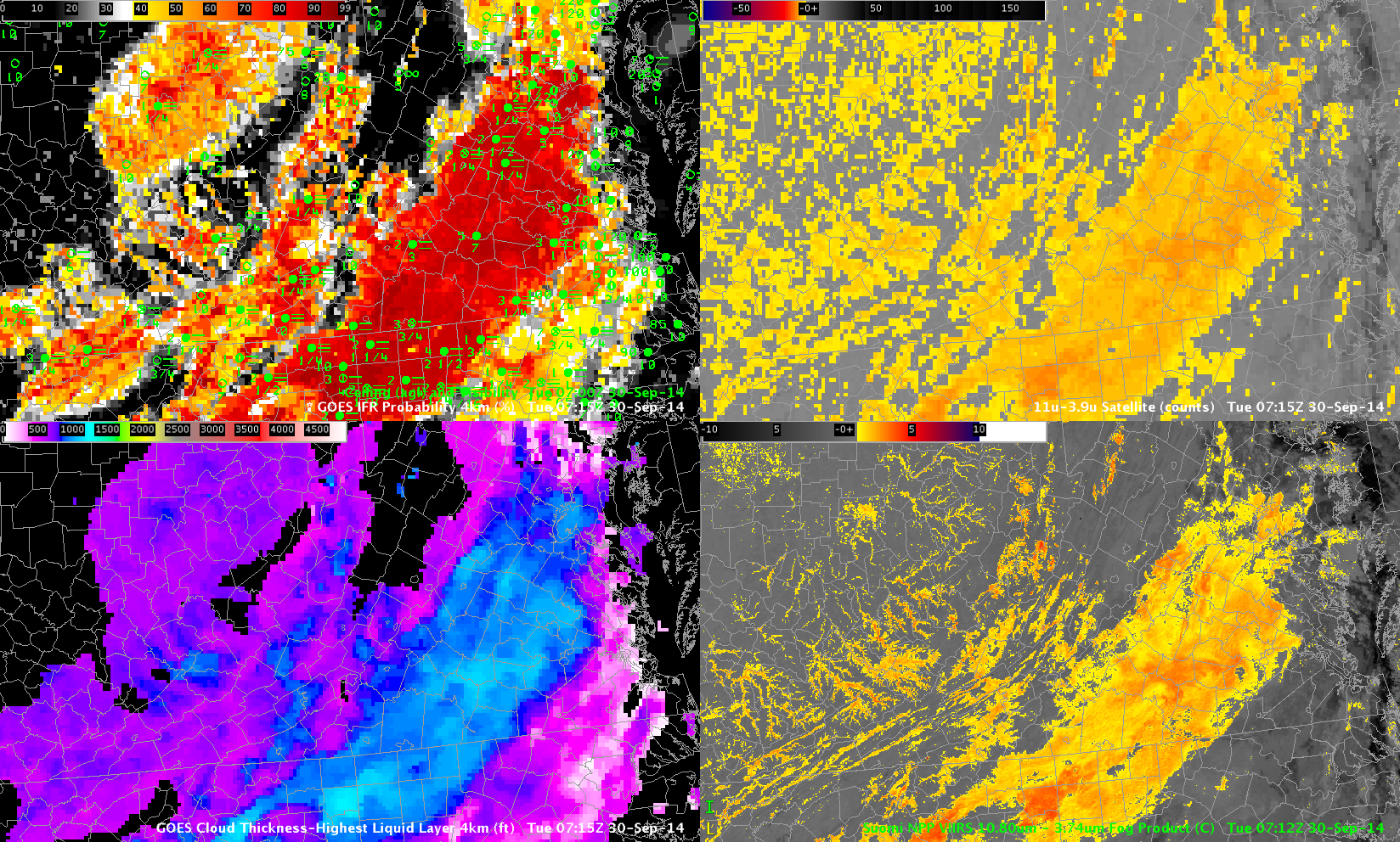
How well did the GOES-R IFR Probability Fields diagnose this fog event? Note the presence of high and mid-level clouds in the picture at top, from the morning of 12 November. Their signature should be in the IFR Probability fields as well, and that is the case.

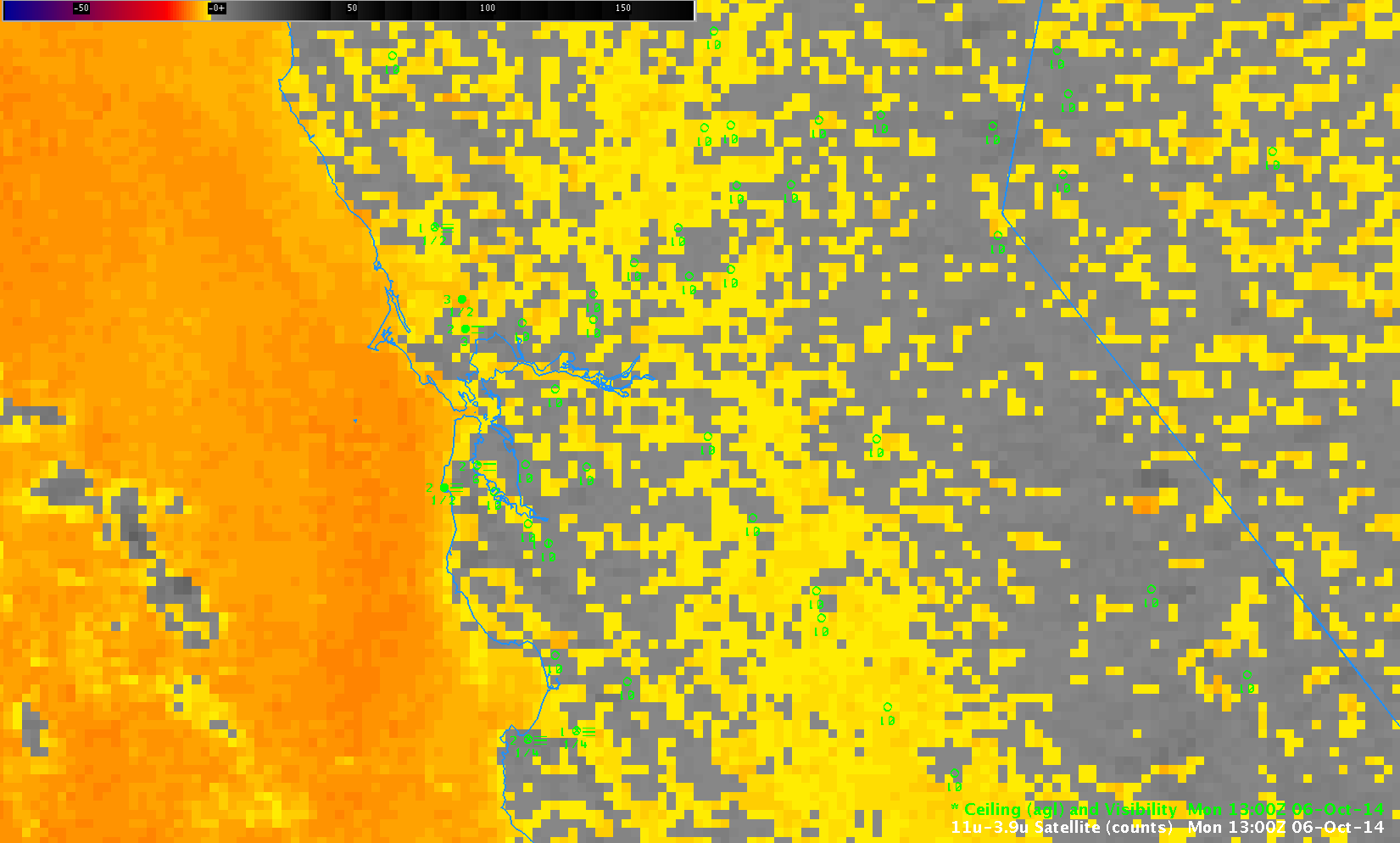
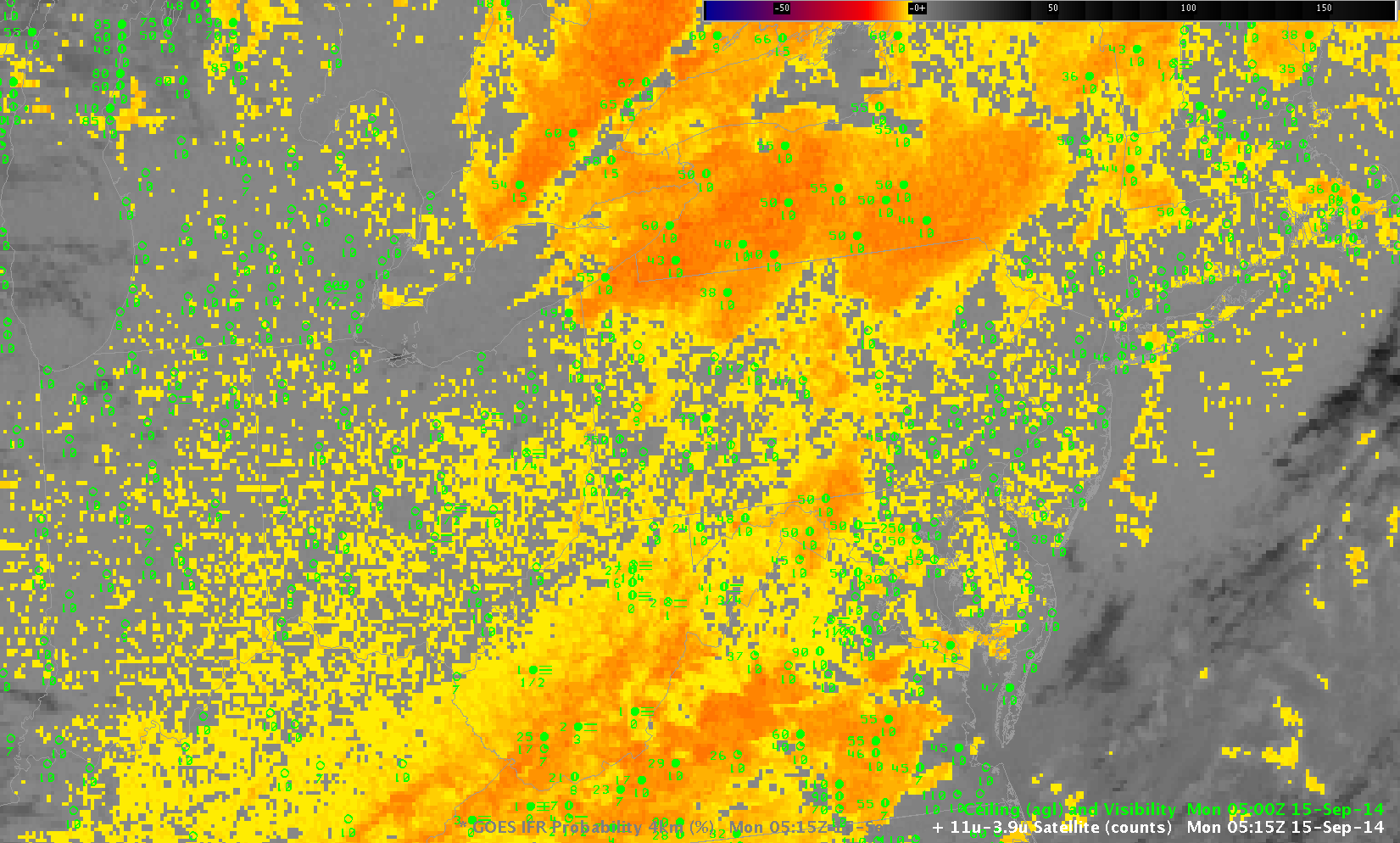
GOES-R IFR Probabilities (Upper Left), GOES-East Brightness Temperature Difference (10.7 µm – 3.9 µm) (Upper Right), GOES-R Cloud Thickness (Lower Left) and GOES-R Low IFR Probability (Lower Right) (Click to animate)

In the animation above, the effect of high clouds is obvious on the IFR (and Low IFR) Probability fields: when mid-level or high clouds prevent satellite data from being used as a predictor in IFR Probability fields, then model data are the main predictors. Model data have coarse resolution relative to satellite data so the IFR Probability fields in those regions have a smoother look that is not at all pixelated. Note how a signal in of low clouds in the Brightness Temperature Difference Field (orange or yellow enhancement) nearly overlaps the more pixelated parts of the IFR and Low IFR Probability fields. Where cirrus/mid-level clouds are indicated in the brightness temperature difference fields, IFR and Low IFR Probability fields are smoother; these are also regions where the GOES-R Cloud Thickness (which field is of the thickness of the highest water-based cloud viewed by the satellite) is not computed because ice-based clouds are screening any satellite view of water-based clouds.

Note how southeastern Massachussetts in the animation above — under multiple cloud layers — has relatively small IFR and low IFR (LIFR) Probability values in a region where dense fog is reported. This arises because the model being used — the Rapid Refresh — to generate IFR Probability predictors is not saturating in the lower levels. It is important to remember that when satellite data are missing, only model data are used to generate GOES-R Fog/Low Stratus products. To rely on only the IFR Probability fields as an indication of the presence of fog is to believe the model simulation in that region is correct. Sometimes the model simulation is correct (this case, for example); in the present case, however, there were regions in southeastern Massachusetts where the model forecast did not accurately represent the observed conditions.

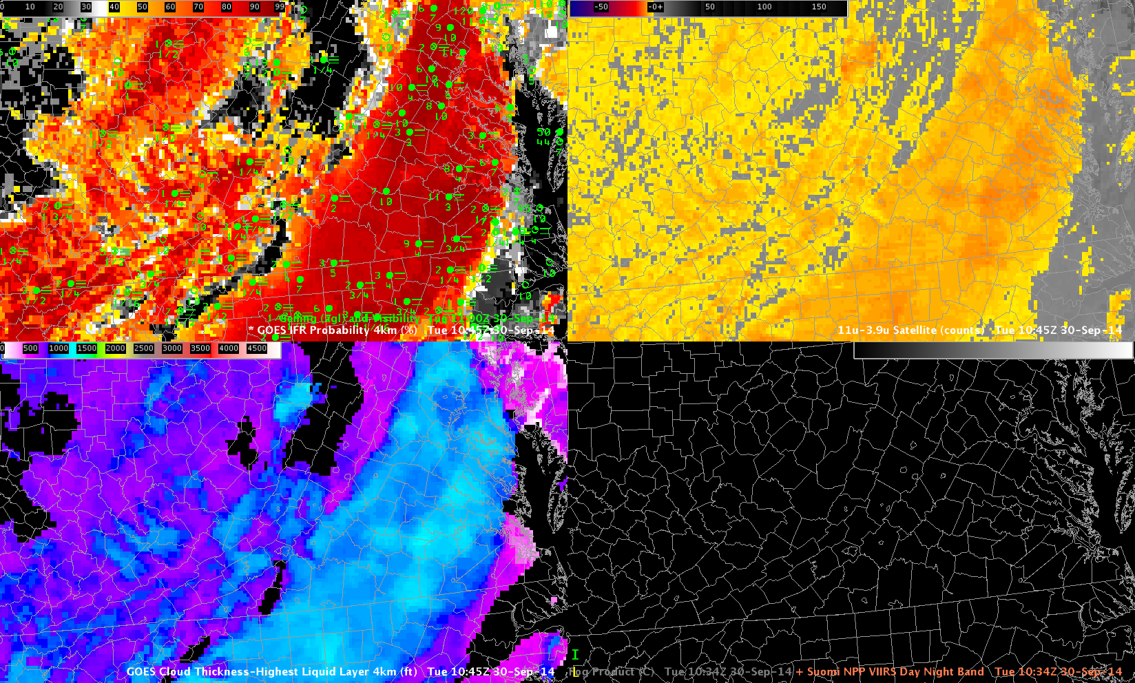
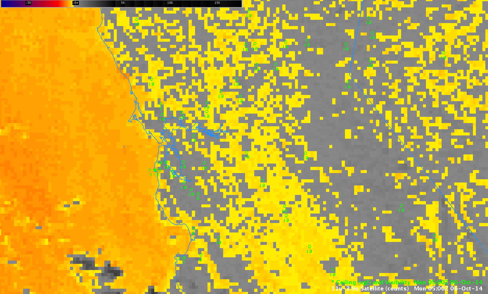
Suomi NPP overflew New England around 0700 UTC on 12 November, and the data collected are included in the image toggle below. Suomi NPP better resolves some of the smaller valleys in interior New England, and some of the sharp edges to the fields.

As above, but with a toggle between Suomi NPP VIIRS Day Night Band and Brightness Temperature Difference (11.45 µm – 3.74 µm) in the lower right. All data at ~0700 UTC 12 Nov (Click to enlarge)

Fog near Hanford California

Tweeted Message from the National Weather Service in HNX (Hanford, CA) showing GOES-R IFR Probabilities in the central Valley of California (click to enlarge)

The National Weather Service in Hanford tweeted the image, above, of IFR Probability this morning. How did the evolution of IFR Probabilities compare to that of brightness temperature difference fields?

The hourly animation, below, suggests that data from the Rapid Refresh model was likely crucial in determining exactly where the lowest visibility occurred; the brightness temperature difference field did not capture the horizontal extent of the narrow band of fog that developed to the east of Interstate 5 (The interstate is the purple line in the animation). Indeed, the brightness temperature difference field appears to offer little in the way of forecast value, and differences trend to zero as the sun starts to rise at the end of the animation. In contrast, both IFR and LIFR Probabilities have peak values where ceilings are obscured and visibilities are near zero, in and around Hanford, and those large values persist through sunrise.

Hourly GOES-R IFR Probabilities (Upper Left, computed with data from GOES-15) with ceilings and visibilities plotted, Hourly GOES-R LIFR Probabilities computed with data from GOES-15 (Lower Left), GOES-15 Brightness Temperature Difference (10.7µm – 3.9µm) (Upper Right), Suomi NPP Day Night Band and Brightness Temperature Difference (11.45µm – 3.74µm) (Lower Right), times as indicated (Click to enlarge)

Suomi NPP overflew the central Valley at 0938 UTC. The Day Night Band and the brightness temperature difference (11.45µm – 3.74µm) field, below, do not contain signatures of dense fog near Hanford.

As above, but at 0945 UTC, when Suomi NPP data were present (Click to enlarge)

The two-hour time-lapse video, below, shows the evolution of the Fog at the National Weather Service Office in Hanford on the morning of 4 November.

Fog over the Ozarks and southern Plains

GOES-IFR Probabilities, computed from GOES-13 and Rapid Refresh, hourly from 0100 through 1300 UTC on 21 October 2014 (Click to enlarge)

Fog and stratus developed overnight over the Ozark Mountains and southern Plains. The hourly loop of GOES-R IFR Probabilities shows the development and expansion of visibility and ceiling reductions over the area. How do these fields compare to other measures of fog? Brightness Temperature Difference fields, below, generally overestimate the regions of fog. The 0200 and 0800 UTC brightness temperature difference fields, below, are toggled with the IFR Probabilities; the inclusion of surface information via the Rapid Refresh Model correctly limits the positive brightness temperature difference to regions where fog and low stratus are most likely. The satellite-only signal overpredicts regions of reduced visibilities because it can only see the top of the cloudbank; this offers little information about the cloud ceilings!

GOES-13 Brightness Temperature Difference (10.7 µm – 3.9 µm) and GOES-based IFR Probabilities at 0200 UTC, 21 October 2014 (Click to enlarge)

GOES-13 Brightness Temperature Difference (10.7 µm – 3.9 µm) and GOES-based IFR Probabilities at 0800 UTC, 21 October 2014 (Click to enlarge)

Brightness Temperature Difference fields are occasionally contaminated by stray light in the signal. This happened on 21 October at 0400 UTC. The Brightness Temperature Difference fields at 0345, 0400 and 0415 UTC are shown below, with the GOES-R IFR Probabilities for the same time follow. Note how Stray Light contamination does bleed into the GOES-R IFR Probability field; if there is a large change over 15 minutes in the IFR Probability signal, consider the possible reasons for that change. Stray light contamination is a strong candidate if the signal is near 0400-0500 UTC with GOES-East. There are regions in the IFR Probability fields where even the strong — but meteorologically unimportant — brightness temperature difference signal during stray light is not enough to overcome the information from the Rapid Refresh model that denies the possibility of low-level saturation (for example, in northern Kansas or southern Oklahoma).

GOES-13 Brightness Temperature Difference (10.7 µm – 3.9 µm) at 0345, 0400 and 0415 UTC, 21 October 2014 (Click to enlarge)

GOES-based IFR Probabilities at 0345, 0400 and 0415 UTC, 21 October 2014 (Click to enlarge)

MODIS data from either Terra or Aqua can give important early alerts to the development of Fog/Low Stratus. Because of its superior resolution to GOES, the character of the developing fog can be depicted with more accuracy. The MODIS-based IFR Probability, below, in a toggle with the GOES-based IFR Probability at the same time, distinctly shows that the fog development at 0430 UTC is starting in the small valleys of the Ozarks of northwest Arkansas. GOES-based IFR Probabilities give a broader signal; certainly if you are familiar with the topography of the WFO you can correctly interpret the coarse-resolution GOES data, but the MODIS data spares you that necessity.

GOES- and MODIS-based IFR Probabilities at ~0430 UTC, 21 October 2014 (Click to enlarge)

Suomi NPP data can also be used to compute IFR Probabilities, but those data are not yet computed for AWIPS. The Ozarks were properly positioned on 21 October to be scanned by two successive orbits of Suomi NPP (one of the benefits of Suomi NPP’s relatively broad scan), and the brightness temperature difference fields (11.45µm – 3.74µm) at 0715 and 0900 UTC are shown below. As with MODIS, the strong signal in the river valleys is apparent. (The Day Night band from Suomi NPP for this event does not show a strong signal because the near-new Moon provides no illumination at 0745 or 0900 UTC: it hasn’t even risen yet.)

Suomi NPP Brightness Temperature Difference (11.45 µm – 3.74 µm) and 0715 and 0900 UTC, 21 October 2014 (Click to enlarge)

Successive Suomi NPP Scans Show Stratus/Fog movement

Suomi NPP Day/Night Band at 0926 and 1106 UTC on 9 October 2014 (Click to enlarge)

(A Blog post on Suomi NPP Imagery over the western US from 10 October is available here).

Polar orbiters typically don’t give good temporal resolution, especially near the Equator. In mid-latitudes, however, Polar Geometry can yield views over a wide area on two successive scans. This happened along the West Coast early in the morning on 9 October. Two regions show noticeable changes in stratus between the two times: stratus/fog extends farther down the Salinas Valley at the southern edge of image, and stratus/fog expands over southwestern Puget Sound in Washington. The Brightness Temperature Difference field (11.35µm – 3.74µm) from Suomi NPP for the same times shows a similar evolution over the Salinas Valley, but the view of Washington is obscured by thin cirrus. These cirrus (that show up as black enhancements below) are mostly transparent in the Day Night Band but not in the infrared bands.

Suomi NPP Brightness Temperature Difference (11.35µm – 3.74µm) at 0926 and 1106 UTC on 9 October 2014 (Click to enlarge)

MODIS instruments onboard Terra and Aqua yield spectral data that can be used to generate GOES-R IFR Probability Fields. The animation below shows high-resolution imagery of where IFR Probabilities are highest, but only at three distinct times: 2152 UTC on 8 October and 0537 and 0949 UTC on 9 October. An increase in IFR Probabilities around Monterey Bay is apparent (and consistent with the Suomi NPP Observations above); IFR Probabilities also increase along the Oregon Coast and around Puget Sound.

MODIS-based GOES-R IFR Probabilities at 2152 UTC 8 October, 0547 UTC 9 October and 0949 UTC 9 October (Click to enlarge)

How do GOES-based observations complement the Polar Orbiter data above?

GOES-15 based GOES-R IFR Probabilities, hourly from 0200 through 1400 UTC, 9 October 2014 (Click to enlarge)

The hourly animation above shows the slow increase of IFR Probability in/around Monterey Bay, and also a push of higher IFR Probability onto the Oregon Coast that occurs after the last MODIS-based IFR Image shown farther up. (Higher IFR Probabilities also spill into San Francisco Bay). Do surface observations of ceilings and visibilities agree with the IFR Probability fields? The loops below, from Oregon (below) and Monterey Bay (bottom) suggest that they do. For example, Eugene OR (and stations north and south of Eugene) show IFR conditions as the high IFR Probability field moves in after 1100 UTC. GOES-based data is valuable in monitoring the motion of IFR Probability fields; keep in mind, though, that small-scale features may be lost. For example, it is difficult for GOES to resolve the Salinas Valley.

GOES-15 based GOES-R IFR Probabilities, hourly from 0200 through 1500 UTC, 9 October 2014, with surface and ceiling observations superimposed (Click to enlarge)

GOES-15 based GOES-R IFR Probabilities from 0400 through 1400 UTC, 9 October 2014, with surface and ceiling observations superimposed (Click to enlarge)

IFR Probability along the West Coast

MODIS data from Terra and Aqua, Suomi NPP data, and GOES-15 data yield different types of information that can be used to observe clouds in a region. Probabilities of IFR conditions — that is, what’s going on at cloud base, which is a part of the cloud the satellite cannot see — can be produced by combining satellite observations of cloud tops and data from a model (such as the Rapid Refresh) that includes accurate predictions low-level moisture.

GOES-based IFR Probabilities (Upper Left), GOES-15 Brightness Temperature Difference (10.7µm – 3.9µm) (Upper Right), MODIS-based IFR Probabilities (Lower Right) at 0646 UTC, 0919 and 1058 UTC (Click to enlarge)

The three MODIS images, above (bottom right), show the slow encroachment of higher IFR Probabilities east-southeastward along the Sonoma/Marin county border. The high-resolution imagery from MODIS allows a more accurate depiction of the sharp edges that can occur as marine stratus penetrates inland around topographic features. MODIS data also suggests reduced ceilings in San Francisco.

As above, but at 0919 UTC only, with a toggle of MODIS Brightness Temperature Difference (11µm – 3.7 µm) and IFR Probability (Bottom Right) (Click to enlarge)

The 0919 UTC MODIS pass (from Aqua) happened to pass at a time when the GOES-West brightness temperature difference field was contaminated by stray light. The toggle above shows the difference between MODIS and GOES Brightness Temperature Difference fields at that time. MODIS is only detecting a signal where low clouds are present (or where soil differences allow the emissivitiy differences that can show up in the brightness temperature difference field, in this case over Nevada)

Suomi NPP overflew California at 1000 UTC, and those images are below. The brightness temperature difference field, and the Day Night band show clouds offshore, and city lights in and around San Francisco Bay and Monterey Bay. Regions of stratus have moved inland towards southern Sonoma County, over San Francisco, and over Monterey. There is a slight brightness temperature difference signal in the Suomi NPP data that extends down the Salinas Valley as well; it’s difficult to perceive cloudiness in the Day Night band in that region however.

As above, but with a toggle of Suomi NPP Brightness Temperature Difference and Day Night Band in the lower left, data at 1021 UTC (Click to enlarge)

The great strength of GOES data is its ability to monitor continuously the West Coast. Trends are therefore more easily observed. The hourly loop, below, shows that along much of the west coast, marine stratus stayed off shore through the night. Higher IFR Probabilities are also confined to regions where ceilings and visibilities were reduced. This is an improvement on the brightness temperature difference fields for the same time that have strong signals over much of the central Valley (for example, at 0500 and 1300 UTC, as well as at 0915 UTC, above).

GOES-15 IFR Probabilities, hourly from 0400 through 1300 UTC, 6 October 2014 (Click to enlarge)

MODIS vs. GOES-based IFR Probabilities

MODIS-based and GOES-based IFR Probability fields at ~0300 UTC on 03 October 2014 (click to enlarge)

A great benefit of a polar-orbiting satellite, such as Terra, or Aqua, or Suomi NPP, is that they provide very high-resolution imagery. The toggle above shows the early development of overnight fog over the mountainous terrain of Pennsylvania. The MODIS IFR Probability resolves with clarity the small river valleys of north-central Pennsylvania. Both MODIS and GOES suggest higher probabilities over the elevated terrain (the Laurel Highlands near Johnstown and regions around Bradford). A later overpass, below, just after 0700 UTC, shows the expansion of the regions of high probability has occurred in both MODIS and GOES-based products, but the MODIS-based product continues better to resolve the river valleys, such that Probabilities are higher over River Valleys (over the Pine Creek basin of north-central Pennsylvania, for example).

MODIS-based and GOES-based IFR Probability fields at ~0700 UTC on 03 October 2014 (click to enlarge)

Suomi NPP also provides high-resolution imagery, and sometimes orbital geometry allows two consecutive orbits – about 90 minutes apart — to view the same region, as below over Pennsylvania. This also shows the general increase in fog/low stratus over the eastern two-thirds of the state. (IFR Probability algorithms do not yet include Suomi NPP data).

Suomi NPP Brightness Temperature Difference (11.35µm – 3.74µm) Fields at 0617 and 0756 UTC 03 October 2014 (click to enlarge)

Polar orbiters lack good routine temporal resolution, a shortcoming that can be a significant drawback. For example, none of the satellites are overhead just before sunrise, a time when the start of the morning commute might demand information. For that, GOES data (with its 15-minute temporal resolution) is essential. The 1145 UTC image, below, shows IFR Probabilities over the region at that time, and GOES data are routinely used to monitor the evolution of IFR Probability fields over the course of the night.

GOES-based IFR Probability fields at 1145 UTC on 03 October 2014 (click to enlarge)

Fog over the Piedmont of Virginia

GOES-R IFR Probabilities (Upper Left), GOES-R Cloud Thickness (Lower Left), Brightness Temperature Differences from GOES-13 (Top Right, 10.8 µm – 3.9 µm) and from Suomi-NPP (Bottom Right, 11.35 µm -3.74 µm , all at 0715 UTC 30 September (Click to enlarge)

Radiation fog developed over the Piedmont of Virgina on the morning of 30 September in a region with little pressure gradient. The image above, from 0715 UTC, shows IFR Probability to be very high (from 85-95%) over the Virginia Piedmont. Numerous stations in the region were reporting IFR visibilities and ceilings. Brightness Temperature Difference products are also highlighting the region (Note the advantage in the Suomi NPP Brightness Temperature Difference field that ably captures fine detail related to Ridge/Valley topography over the Appalachians); the advantage of IFR Probability fields is that it includes surface information so that someone using the field can be more certain that the stratus detected by the satellite is in contact with the ground as fog. The animation below shows the evolution of the fields from 0200 through 0700 UTC.

As above, but with Suomi NPP Day/Night band in lower Right. Hourly imagery from 0200 through 0700 UTC on 30 September 2014 (Click to enlarge)

GOES-R Cloud Thickness (the thickness of the highest water-based cloud) can be used to estimate when fog/low clouds will burn off. The estimate is most accurate for strict radiation fog. GOES-R Cloud Thickness is only computed for water-based clouds during non-twilight times (in other words, it is not computed in the hours surrounding twilight at both sunrise and sunset). The last value of Cloud Thickness before morning twilight (shown below) can be used in concert with this scatterplot to guess when clouds might dissipate. Values over eastern Virginia, near Richmond, exceeding 1100 feet, correspond to a dissipation time 4+ hours after 1100 UTC, or at 1500 UTC. In this case, that value was an underestimate.

As above, but for 1100 UTC 30 September 2014

GOES-13 Visible imagery, hourly between 1215 and 1715 UTC 30 September 2014 (Click to enlarge)

Comparing IFR Probabilities and Brightness Temperature Differences over Wisconsin

GOES-R IFR Probabilities computed from GOES-East (Upper Left), GOES-13 Brightness Temperature Difference (10.7 µm – 3.9 µm) (Upper Right), GOES-R Cloud Thickness computed from GOES-East (Lower Left), GOES-R IFR Probabilities computed from MODIS (Lower Right), hourly from 0300 through 1200 UTC 26 September (Click to enlarge)

Fog developed over southeast Wisconsin during the morning of 26 September 2014. The GOES-R IFR Probability fields did a better job of detecting the hazard than did the traditional method of satellite-based fog detection (brightness temperature difference) in part because of the presence of higher clouds. (Fog/low stratus also generated IFR conditions over northeast Ohio). The animation above also includes a MODIS-based IFR Probability field. In fact, three separate MODIS-based fields were created, one at 0430 UTC, one at 0700 UTC, and one at 0845 UTC, shown below (Note that the MODIS-based IFR toggles with the MODIS Brightness Temperature Difference field). MODIS data confirms the small-scale nature of the fog event over southeast Wisconsin. (Note also how the MODIS-based data at 0700 UTC, below, are able to resolve the small river valleys in Pennsylvania in ways the GOES data cannot.)

Note how the IFR Probability fields ignore regions of mid-level stratus, such as over northeast Ohio along Lake Erie.

As above, but for 0430 UTC, and with the MODIS Brightness Temperature Difference in the lower right (Click to enlarge)

As above, but for 0700 UTC, and with the MODIS Brightness Temperature Difference in the lower right (Click to enlarge)

As above, but for 0845 UTC, and with the MODIS Brightness Temperature Difference in the lower right (Click to enlarge)

Suomi NPP Overflew the region as well. GOES-R IFR Probability algorithms do not yet incorporate Suomi NPP data; when that happens, an early morning snapshot that complements MODIS overpasses will be available.

As up top, but with Suomi NPP Brightness Temperature Difference (11.35 µm- 3.74 µm) in the bottom right, times at 0647 and 0831 UTC 26 September (Click to enlarge)

Stratus and Fog over the northeast and mid-Atlantic States

GOES-13 Color-Enhanced Brightness Tempreature Difference Fields (10.7 µm – 3.9 µm), hourly from 0200 through 1100 UTC, 15 September 2014 (Click to enlarge)

Brightness Temperature Difference Fields from GOES-13 show large regions over Pennsylvania and surrounding states during the early morning hours of September 15th. (Note that the image at 0515 UTC, not in the loop above, shows the effect of stray light). If you look at the ceilings and visibilities in the imagery above, you will note that many regions where stratus/fog are indicated by the brightness temperature difference field (over upstate NY, for example), do not in fact show anything near IFR conditions. Always recall that the satellite is seeing the top of the cloud deck; whether or not that cloud extends to the surface is beyond the capability of present satellite systems. (You can infer it sometimes, of course, especially if the signal is confined to a narrow river valley, as occurs in the animation above: The Ohio River along the northern panhandle of West Virginia shows up very well).

GOES-13 IFR Probability Fields, hourly from 0200 through 1100 UTC, 15 September 2014 (Click to enlarge)

IFR Probability fields for the same time do a better job of highlighting only where reduced ceilings and visibilities are present. For example, the region of stratus over upstate New York is screened out, as well as the region over southern and southeastern Virginia. Probabilities are also quite high over the Ohio River Valley, where river fog is likely occurring. Note that IFR Probabilities over southwestern Indiana at the end of the animation have the characteristic look (a flat field) associated with IFR Probabilities created without the benefit of satellite data.

MODIS data were able to provide a a high-resolution image of this scene in the middle of the night. As with GOES, MODIS identified the large region of stratus over upstate New York and over southeastern Virginia, and the IFR Probabilities correctly screened out those stratus clouds. River Valleys show up distinctly along the Ohio River downriver from Pennsylvania; smaller IFR Probabilities surround the rivers. Sometimes MODIS data can give an early alert to the development of fog; in the present case, when MODIS overflew the region, fog development was at sufficiently large a scale that GOES-13 could also detect it.

MODIS Color-Enhanced Brightness Tempreature Difference Fields (11 µm – 3.9 µm) and IFR Probability Fields at 0722 UTC 15 September 2014 (Click to enlarge)

Suomi NPP data also viewed the developing river fogs, both in the day/night band, and in the brightness temperature difference (11.35 µm – 3.74 µm), below. At present, IFR Probabilities are not computed from Suomi NPP satellite data.

Suomi NPP Color-Enhanced Brightness Tempreature Difference Fields (11.35 µm – 3.74 µm) and Day Night band visible imagery at 0653 UTC 15 September 2014 (Click to enlarge)

IFR Probabilities over the Texas Panhandle

GOES_MODIS_IFR_SNPP_BTD-DNB_0930UTC_02Sep2014

GOES-R IFR Probabilities (Upper Right), GOES-13 Brightness Temperature Difference (10.7 µm – 3.9 µm) (Upper Left), MODIS IFR Probabilities (Lower Left), Suomi NPP Brightness Temperature Difference (11.35 µm – 3.74 µm) and Day Night Band (Lower Right), all near 0930 UTC 2 September 2014 (Click to enlarge)

GOES-R IFR Probabilities (from GOES and from MODIS) over the Great Plains and southern Rockies indicated one region where IFR conditions were most likely: over the Texas panhandle, where IFR conditions were reported. There is a strong signal in the GOES-based Brightness Temperature Difference field there (and in the Suomi NPP Brightness Temperature Difference field) as well. There is also a Brightness Temperature difference signal in regions where IFR conditions are not occurring; in those locations, stratus is present, or (over the Rockies) emissivity differences in the dry soil are present, both of which conditions will lead to a signal in the brightness temperature difference that is unrelated to surface visibility and ceilings. This is therefore another example showing how incorporation of model data that accurately describes saturation (or near-saturation) in the lowest model layers can help the GOES-R IFR Probability more accurately depict where IFR conditions are present.

GOES-R Fog Product Examples

Fog detection fusing GOES, Terra/Aqua or Suomi/NPP Satellite data with Model output