Category Archives: Plains

Fog over Kansas

GOES_IFR_PROB_20130917_0832

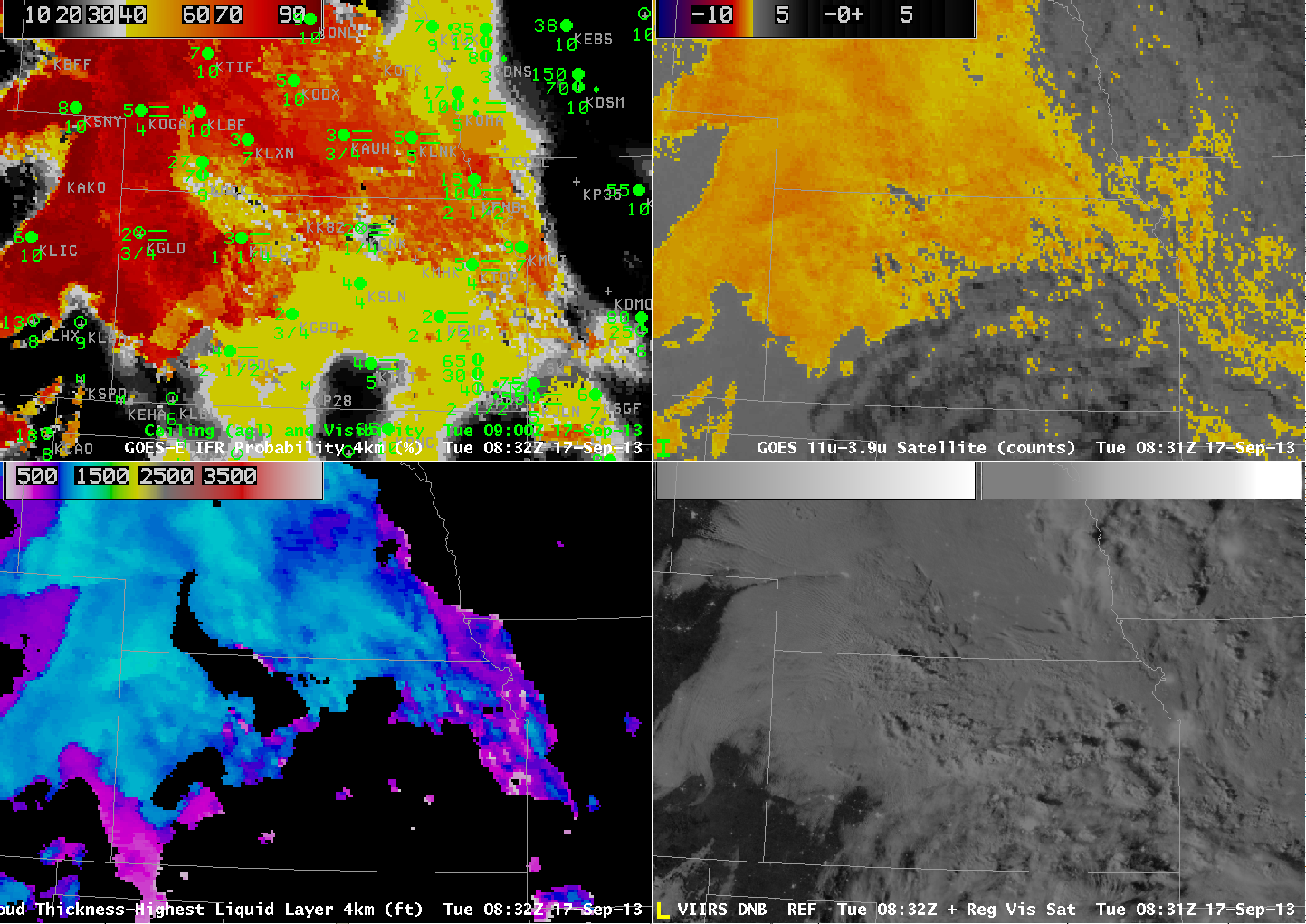
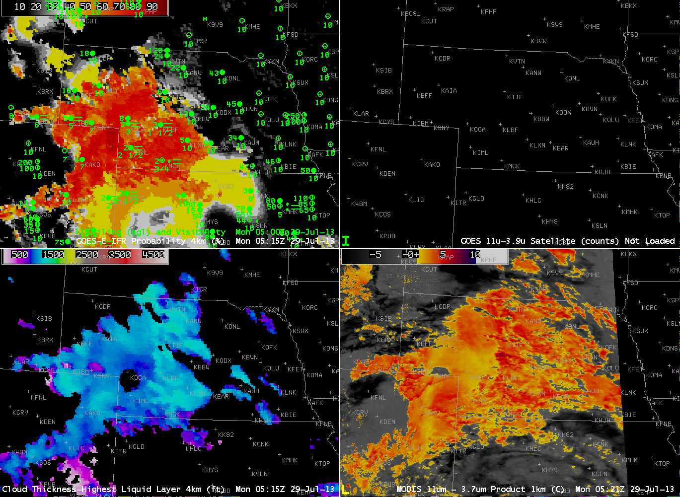
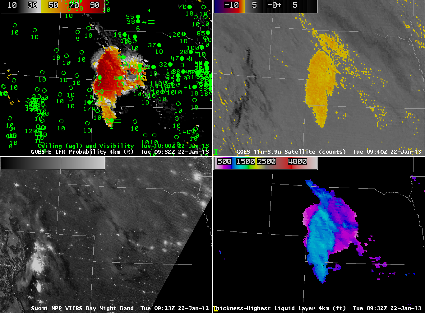
GOES-R IFR Probability (Upper Left), GOES-East Brightness Temperature Difference (Upper Right), GOES-R Cloud Thickness (Lower Left), Suomi/NPP Day/Night Band (Lower Right), all imagery at ~0830 UTC on 17 September 2013 (click image to enlarge)

Light winds with a small upslope component allowed for the formation of fog over the High Plains on the morning of 17 September 2017. The image above shows the GOES-R IFR Probability, GOES-East Brightness Temperature Difference (10.7 µm – 3.9 µm), the GOES-R Cloud Thickness and the Day/Night band from Suomi/NPP that provides for nighttime visible imagery. In the imagery above, a large region over southeastern Kansas is overlain by higher ice-based clouds (likely cirrus) such that the brightness temperature difference product does not give the signal that is common with fog and low stratus (in the enhancement used here, fog and low stratus occur where the brightness temperature difference is colored orange or yellow). The Day/Night band visible imagery also suggests high clouds over southeast Kansas. Surface observations do show reduced visibilities, at or near IFR conditions. In this region, the IFR Probability Product gives useful information by using Rapid Refresh Data to diagnose the possibility of low-level fog. The probabilities are smaller — in the 40- to 50% range — but that is because no satellite data are being used as predictors. IFR Probabilities are very high only if both predictors — satellite and Rapid Refresh — are associated with high probability of fog/low stratus.

Note also how the Cloud Thickness product yields no information where high clouds are present. The Cloud Thickness is the thickness of the highest liquid cloud layer; the presence of ice clouds or mixed phase clouds precludes the determination of how thick a water cloud is because the satellite cannot view the water-based cloud.

GOES_IFR_PROB_20130917_1215

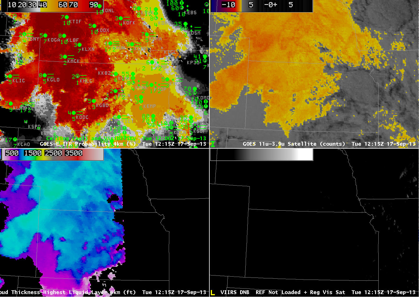
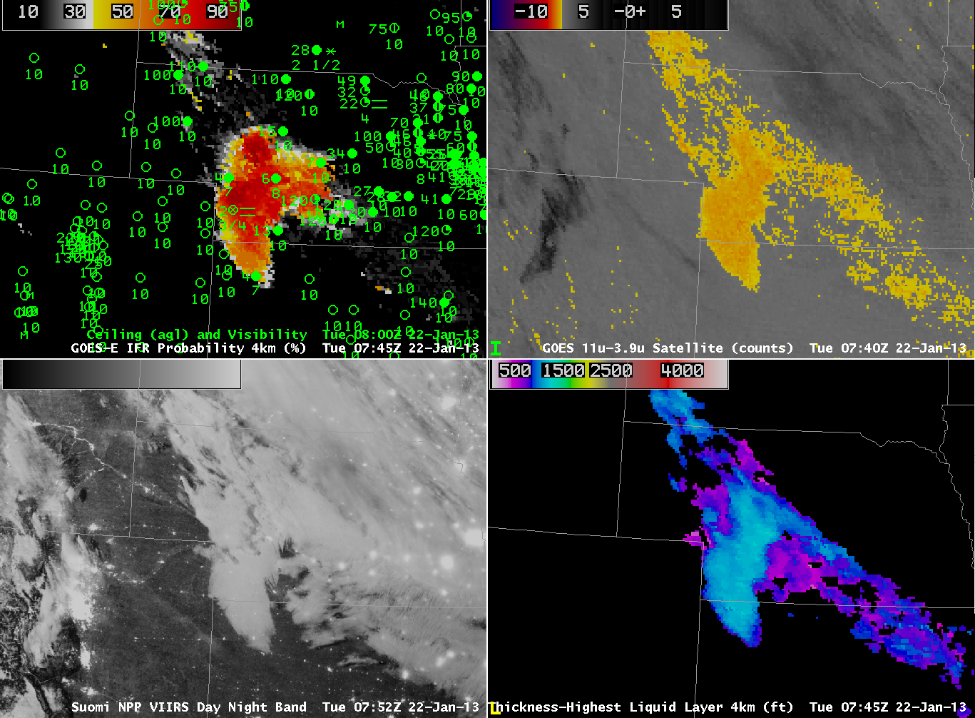
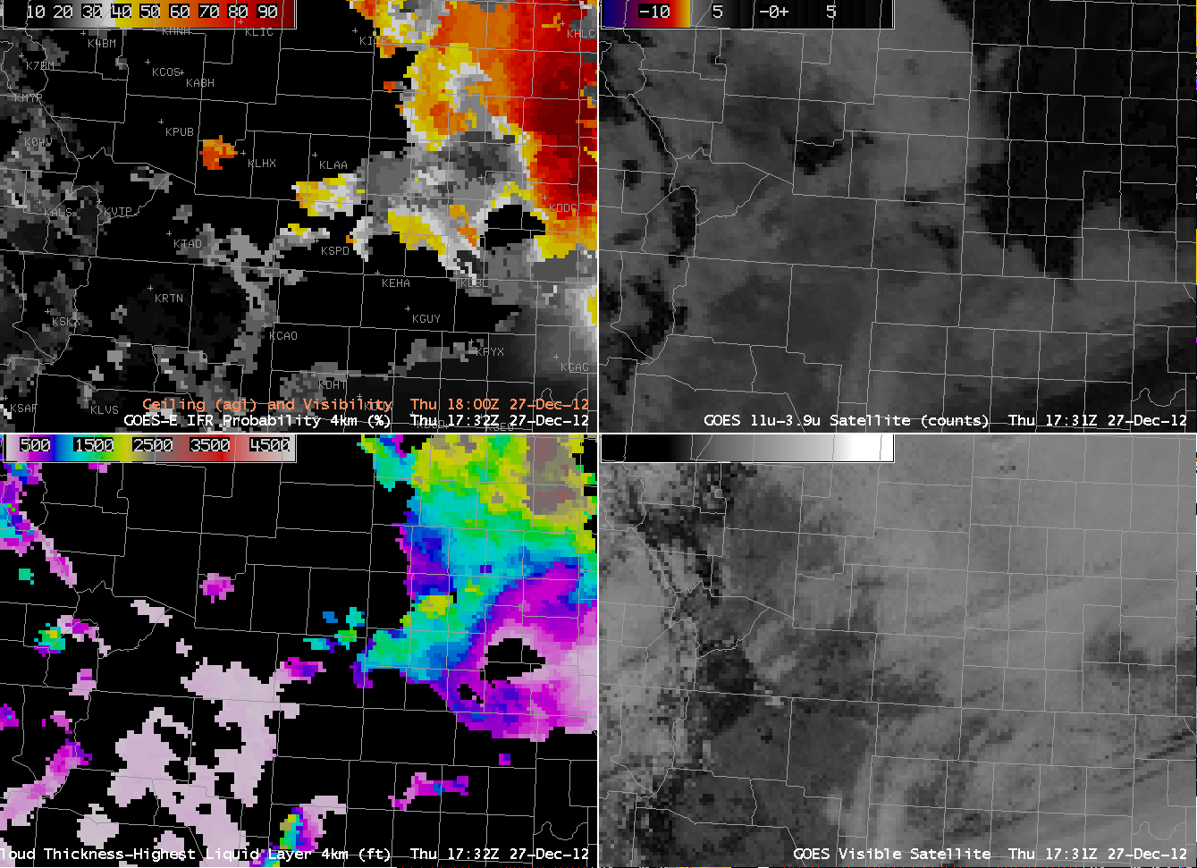
As above, but at 1215 UTC (click image to enlarge)

The 1215 UTC image shows the effect of twilight conditions moving westward across Kansas — GOES-R Cloud Thickness is not computed during twilight conditions that occurring over eastern Kansas, although they are still computed around Dodge City, where the computed cloud thickness is just over 1000 feet thick. The 1200 UTC Sounding from Dodge City, below, does show a nearly-saturated layer at the surface (about 927 mb, or about 2700 feet ASL) up to about 870 mb (4600 feet ASL).

KDDC_20130917_1200

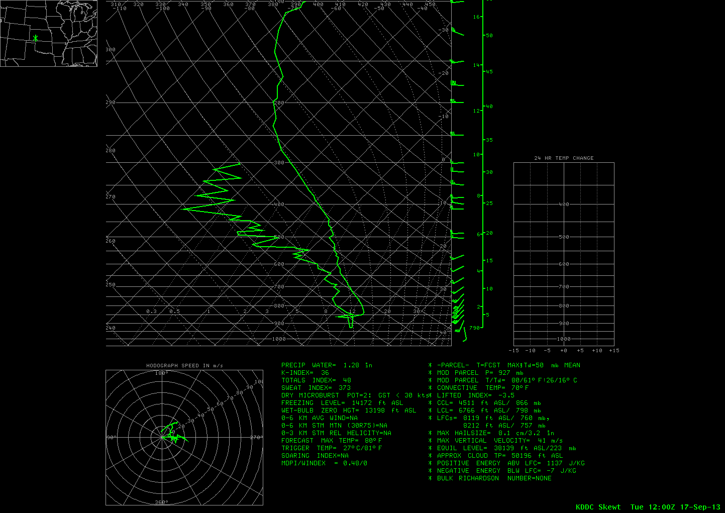
Upper Air Sounding from Dodge City, KS, 1200 UTC (click image to enlarge)

Fog Detection under Cirrus

MODIS Brightness Temperature Difference and MODIS-based GOES-R IFR Probabilities, 30 July 2013, 0835 UTC

MODIS Brightness Temperature Difference and MODIS-based GOES-R IFR Probabilities, 30 July 2013, 0835 UTC

The toggle above switches between a brightness temperature difference field and a GOES-R IFR Probability field (both from MODIS) over Missouri and Kansas (including the busy airport in Kansas City).  The cirrus shield over the convective complex over Missouri obscures any satellite view of low clouds.  North and west of that cirrus shield, over Nebraska, Kansas and Iowa, the brightness temperature difference indicates clouds comprised of water droplets (that is, stratus or fog).  Ceilings and visibilities underneath the cirrus canopy, and within the stratus deck show regions of IFR conditions. Rapid Refresh model data that is part of the GOES-R IFR Probability algorithm is able to alert a viewer (or forecaster) to the possibility of Fog/Low stratus in areas underneath the cirrus. Probabilities under the cirrus canopy are lower because satellite-based predictors are not used in the computation of probabilities.


Unusual late-July High Plains Fog

GOES_IFR_PROB_20130729_loop

Fog and low stratus developed over the High Plains under easterly (upslope) flow in the early morning hours of July 29, 2013, and the GOES-R IFR Probability fields ably discriminated between regions of stratus and visibility-restricting low stratus/fog.  Note in the imagery above how the Brightness Temperature Difference field (upper right) includes a strong signal over eastern Nebraska where visibility restrictions/low ceilings are not present.  Fusing the satellite data with Rapid Refresh model data allows the MODIS and GOES-based GOES-R IFR Probability fields to more accurately depict the regions of low visibilities/ceilings.  Note that the brightness temperature difference product from MODIS, below (Lower Right), also highlights the mid-level stratus over eastern Nebraska.

MODIS_FOG_20130729_0521

GOES-R vs. Heritage GOES Fog Products in Arkansas

GOES-R IFR Probabilities, from GOES-East (0732 UTC) and 0800 UTC Surface observations of visibility and ceilings (Upper Left), GOES-E Brightness Temperature Difference (10.8 µm – 3.9 µm) (Upper Right), GOES-R Cloud Thickness (Lower Left), MODIS-based Brightness Temperature Difference (11µm – 3.74 µm) GOES-R IFR Probabilities computed using MODIS data (Lower Left, 0739 UTC)

IFR conditions developed over Arkansas and surrounding states overnight from 4 into 5 February.  Compare the brightness temperature difference (the traditional fog-detection product) over southeast Arkansas (where IFR conditions are not occurring) and over southwest Arkansas (where IFR conditions are present).  Although the satellite signal is very similar over the region, surface observations are very different.  The GOES-R algorithm distinguishes between the region with IFR conditions (east Texas, western Arkansas, northwest Louisiana) and the region without IFR conditions (southeast Arkansas, northeast Louisiana).

On the flip side, in regions over northeast Arkansas, where the brightness temperature difference product is not showing low clouds, IFR conditions are present, and the GOES-R IFR probability is elevated.

GOES-R Cloud Thickness over Arkansas just before Dawn — note that dawn has arrived over Tennessee and Mississippi

Cloud Thickness just before twilight conditions can be used to predict when radiation fog will burn off, using this scatterplot as a guide.  The maximum thickness over south-central Arkansas is 1350 feet, and that thickness corresponds to 5 hours after sunrise, or sometime after 1800 UTC.  The animation of visible imagery, below, shows that fog/low clouds are lingering over parts of southern Arkansas.

GOES-13 Visible Imagery over Arkansas, times as indicated.

Fog/Low Stratus over the High Plains

Surface Weather Maps, 0300, 0600 and 0900 UTC on 22 January

High Pressure with origins in the Arctic has pushed cold air into the central United States.  The western edge of the cold dome shows as a stationary front that stretches from central Kansas northwestward into Montana and beyond.  During the early morning hours of 22 January, a small region of IFR conditions developed over western Nebraska.  How did the GOES-R Fog products do in describing this region?

GOES-R IFR Probabilities and surface plots of ceilings/visibilities (Upper Left), GOES-East Brightness Temperature Difference (Upper Right), Suomi/NPP Day/Night Band (Lower Left), GOES-R Cloud Thickness (Lower Right) for various times from 0102 through 1102 UTC 22 January 2013

The animation above shows increasing IFR probabilities over southwest and west-central Nebraska over the course of the night in a region where IFR conditions are developing.  Note how the IFR probabilities are not enhanced in regions where the traditional brightness temperature difference product does have a signal — over eastern Nebraska and northeastern Kansas.  In these regions, the Rapid Refresh Model fields likely include no saturation in the lowest model layers.  Suomi/NPP Night-time Visible imagery, below, at 0752 UTC and at 0933 UTC also show the extent of the fog and low stratus.   However, it’s impossible to tell from the satellite where the visibility obstructions are most likely — that’s why the model data are important in this fused product.  Note the distinct change in illumination between 0752 UTC and 0930 UTC.  The Waxing Gibbous moon set around 0900 UTC.

As above, but for 0745 – 0800 UTC on 22 January 2013

As above, but for 0930 UTC on 22 January 2013

Two examples from 17 January 2013

GOES-R IFR Probabilities computed from GOES-East, 1700 UTC on 17 January 2013

 The image above shows how IFR probabilities can maximize over higher terrain where mountains rise up into a somewhat uniform cloud deck.  IFR probabilties are highest over the Laurel Highlands of Pennsylvania southward along the spine of the Appalachian Mountains in West Virginia (and also in the highlands of north-central Pennsylvania).  IFR Conditions are reported at K2G4 in Maryland, which is 890 meters above sea level, and near-IFR conditions are present at Johnstown, PA (KJST) and Elkins, WV (KEKN), two stations above 600 meters above Mean Sea Level.  In contrast, KCBE and KW99, Cumberland Maryland and Petersburg, WV, are both lower than 300 m above sea level, and IFR condition are not present there.

GOES-R IFR Probabilities (Upper Left), GOES-East Visible Imagery (Upper Right), GOES-East Brightness Temperature Difference (Lower Left), Suomi-NPP 1.61 µm Reflectivity (Lower Right)

GOES-R IFR probabilities maximized near the Missouri River Valley in eastern Nebraska around mid-day on 17 January 2013.  IFR conditions were reported.  The largest visibility restrictions appear to occur over a band of snow that extended southwest to northeast, roughly parallel to the N. Platte River, and IFR probabilities are highest in that region. The snow band shows up well in the visible imagery, and as a black swath in the 1.61 reflectivity (snow absorbs radiation at 1.61µm).

Predicting the dissipation time of Radiation Fog

GOES-R IFR Probabilities (Upper Left), GOES Brightness Temperature Difference (10.7 µm – 3.9 µm) (Upper Right), GOES-R Cloud Thickness (Lower Left), GOES Visible (0.62 µm) (Lower Right) at 1400 UTC on 27 December 2012.

GOES-R Cloud thickness can be used to predict how long it will take radiation fog and low stratus to burn off after developing overnight.  This case from the high plains of Colorado, on December 27th, is typical.  At 1402 UTC, La Junta Colorado is in a region of enhanced IFR Probability, with 2-mile visibilty and 400-foot ceilings.  The Cloud Thickness at this time, the last image available before twilight conditions, was as much as 1200 feet.  This scatterplot suggests that the fog will be gone in 4-5 hours.  The 1732 UTC image, below, shows the final remnant of low cloud persisting (it was not present at 1815 UTC).  Although difficult to see in the visible imagery, perhaps because of snow-covered ground, it shows up well in both the IFR probability field, the Brightness Temperature Difference field, and the Cloud Thickness field.

As above, but at 1732 UTC.

Stray Light in the GOES-R IFR Fog Product

GOES-R IFR Probabilities (upper left), 10.7 µm – 3.9 µm brightness temperature differences (upper right), 3.9 µm micron brightness temperature (lower left), 10.7 µm micron brightness temperature (lower right)

Stray light occasionally intrudes into the 3.9 µm channel, and that has a big impact on both the brightness temperature difference and therefore on the GOES-R IFR product.  The stray light impact on the 3.9 µm channel is evident at 0531UTC — it does not impact the 10.7 µm channel.  The big impact on the brightness temperature difference translates to a big signal in the GOES-R IFR probabilities.  Note how GOES-R IFR probabilities do not change underneath the high-level cirrus over eastern OK, southern MO and Arkansas:  GOES-R IFR probabilities do not use satellite data in regions of multiple cloud layers, or in regions of ice clouds.

Emissivity properties in a drought

GOES-R IFR Probabilities (upper left), Total Precipitable Water (the so-called ‘Blended Product’) (upper right), 10.7 µm – 3.9 µm Brightness Temperature Difference (lower left), Enhanced Water vapor imagery with surface observations (lower right)

The driving mechanism in the brightness temperature difference product, the heritage method for detecting fog and stratus from satellites, keys on differences in the emissivity of water clouds at 3.9 µm versus the emissivity at 10.7 µm.  Water clouds do not emit 3.9 µm radiation as a blackbody does, but they do emit 10.7 µm radiation almost as a blackbody.

As ground dries out in a drought, its emissivity changes. Those changes are a function of wavelength.  This example is from early morning on 31 August, as the remnants of Isaac slowly spread northward.  The brightness temperature difference shows a strong signal around the cirrus canopy of the storm.  These highlighted regions arcing from Kansas to Illinois have suffered extreme drought all summer.  The satellite signal is so strong in this case over the very dry Earth — because of the changed emissivity properties of the parched Earth — that it cannot be overcome by the model parameters that are used.  As a result, IFR probabilities are high over Indiana and Illinois where no IFR conditions are observed.

Importance of Satellite Data in the GOES-

GOES-R IFR Probabilities over Colorado, Kansas and Nebraska, hourly from 0615 UTC to 1415 UTC on 24 August 2012

The loop above shows the importance of satellite data in the GOES-R Fog product.  Only the Satellite information will have sharp cut-offs that are apparent in this imagery.  (The character of the GOES-R IFR field that is described mostly by model data is apparent in the southeast part of this domain at the beginning of the loop when a convective system is moving eastward out of the domina).  Smoothing in model data typically means that sharp cutoffs will not exist.   Note the visibility in Akron, CO, in the center of the image, agrees very well with the GOES-R IFR field.