Category Archives: MODIS

FLS Advecting Northwest Towards the Eastern Aleutians

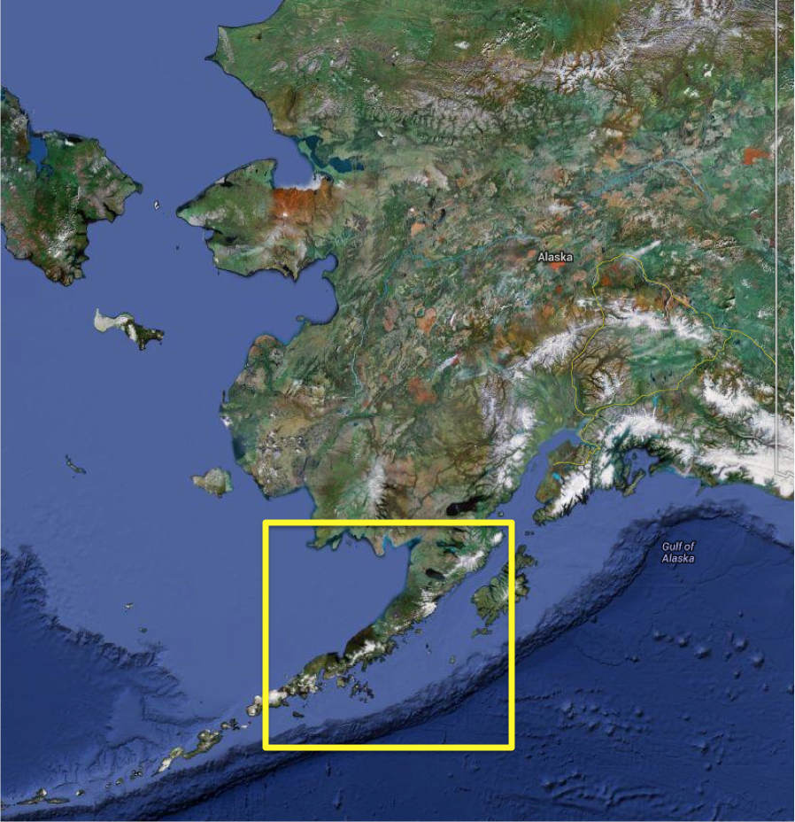
Area of focus in the Eastern Aleutians in Southern Alaska

Due to the location of Alaska, geostationary satellite data can sometimes be difficult to work with. This is because the large satellite angle causes the satellite footprint to increase, thus decreasing the spatial resolution of the data. However, even though the spatial resolution is not ideal the temporal resolution allows geostationary satellite data to remain useful. The example below shows and area of fog/low stratus (FLS) moving northwestward toward the eastern Aleutians in southern Alaska.

GOES-R IFR probabilities computed using GOES-15 (left) and MODIS (right) around 08:20Z on May 30, 2013. Note that the images are rotated so true north is actually oriented from the lower left corner of the images to the upper right corner.

In the image above the orange and darker red colors indicate areas with a high probability of FLS over the northern Gulf of Alaska. The difference in spatial resolution stands out when comparing the images, however, it should be noted that the same areas of higher probabilities in the MODIS image are also picked up in the GOES image, just at a coarser resolution. Although the MODIS image looks more detailed than GOES, temporal trends can not be discerned from a single image. The next available MODIS pass over the area was at 12:26Z.

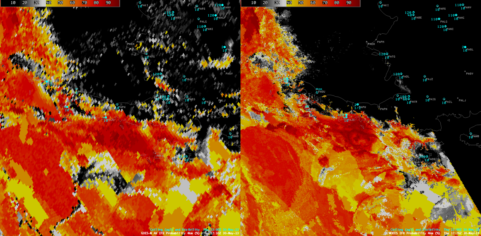
GOES-R IFR probabilities computed using GOES-15 (left) and MODIS (right) around 12:26Z on May 30, 2013. Note that the images are rotated so true north is actually oriented from the lower left corner of the images to the upper right corner. 

In the 12:26Z image the FLS deck moved northwest over the eastern Aleutians as indicated by the higher probabilities that are now over the southeastern side of the Aleutians. This is confirmed by the surface station in Chignik, AK, which reported a ceiling of 400 ft at 12:00Z when it reported no ceiling at 08:00Z. Once both MODIS passes were available the NW movement of the FLS could be observed. However, in the 4 hours between the two MODIS passes it would be hard to forecast whether the IFR conditions would move into the area or stay out at sea.

On the other hand, GOES data was available about every 15 minutes. By animating the GOES images such as this, the slow NW movement of the FLS can be tracked and a better approximation of when IFR conditions will reach the Aleutians can be made. IFR conditions were first reported at Chignik, AK at 09:00Z, just as the higher GOES-R IFR probabilities reached the coastline. Also from the animation, it appears that the eastern Aleutians block the movement of the FLS deck from continuing over to the NW side into the Bering Sea. This blocking might be difficult to interpret from the two MODIS images alone.

Alaska has the largest coastline in the U.S. (more than twice the size of the entire lower 48, including Hawaii) where hazardous areas of FLS can move onshore. Although the high spatial resolution available from MODIS provides more detail in a single scene than GOES, the high temporal resolution that GOES offers makes finding trends in the movement of hazardous low clouds possible. This is another example of how looking at the GOES-R FLS products using GOES and MODIS together can be more useful than using only GOES or MODIS.

Co-registration errors on GOES-14

GOES-R IFR Probabilities computed from GOES-14 (Upper Left), GOES-14 Brightness Temperature Difference (10.7 µm – 3.9 µm) (Upper Right), GOES-R Cloud Thickness (Lower Left), Toggle between MODIS brightness temperature difference (11 µm – 3.7 µm) and GOES-R IFR Probabilities computed from MODIS (Lower Right)

GOES-13 has a co-registration error between the 10.7 and 3.9 µm channel.  That is, the two different channels do not view the same identical pixel.  There is expected to be some variance (at the sub-pixel scale), but the differences exceed system specifications.  This error is also present in GOES-14, as shown above.  The brightness temperature difference product from GOES-14 (upper right) erroneously depicts the presence of Fog/Low Stratus along the western shores of Lakes Michigan and Winnebago and others, and along the various river valleys.  A MODIS image at the same time does not indicate low clouds at all.  The GOES imagery suggests clouds because of the coregistration error:  one channel sees the water and one sees the land, so the difference is actually a land-sea temperature difference rather than one due to emissivity differences between the two wavelengths for water clouds.

The error in GOES propagates into the GOES-R IFR probability fields as a thread of higher probability paralleling the water.  Cloud Thickness fields do not show the signal, however.

This example shows the benefit of using two different satellites to view the same scene.  An misalignment in one typically is not present in the second.

Resolution: MODIS vs. GOES

GOES-R IFR Probabilities computed from GOES-West data (Upper Left), GOES-West Brightness Temperature Difference (10.7 – 3.9 ) (Upper Right), GOES-R IFR Probabilities computed from MODIS data (Lower Left), Toggle between GOES-R Cloud Thickness computed with GOES-West data and with MODIS data, all imagery around 1000 UTC on 13 May 2013

The high spatial resolution on MODIS allows a much more detailed description of IFR probability fields, and cloud thickness fields, than from the GOES-West Imager instrument.  Note in the IFR probability fields on the left, and in the toggle of the Cloud Thickness fields, how the MODIS fields show crisper edges to the fog.  The IFR probability is also — correctly — screening out brightness temperature difference signal in regions where fog and low stratus are not present (in central California and over Nevada).  Note how the three stations reporting IFR conditions all sit within the region where the brightness temperature difference field has a strong signal, and where the IFR Probability is high.

GOES-R Resolution will be between MODIS and present GOES;  that is, nominal pixel size in the GOES-R era will be 2 km.

Radiation Fog over the Allegheny Mountains of Pennsylvania

GOES-R IFR Probabilities computed using GOES-East data, hourly from 0400 UTC through 1000 UTC (excluding 0500 UTC), 26 April 2013

GOES-R IFR Probabilities show a region over the Allegheny Mountains of northwest Pennsylvania slowly acquiring higher and higher probabilities, as ceilings and visibilities drop.  How did this product perform relative to traditional fog detection imagery (the brightness temperature difference product) and relative to data from Polar Orbiting satellites?  (The 0500 UTC imagery is excluded from the animation above because Stray Light Contamination in the 3.9 channel was apparent in the IFR probability fields).

GOES-R IFR Probability computed from GOES-East, 0332 UTC (Upper Left), GOES-East Brightness temperature Difference field (10.7µm – 3.9µm) at 0340 UTC (Upper Right), GOES-R Cloud Thickness (Lower left), GOES-R IFR Probability computed from MODIS data, 0328 UTC (Lower Left).

The ‘traditional’ method of fog detection that exploits emissivity difference of water clouds at 10.7µm and 3.9 µm, upper right in the figure above, at about 0330 UTC, just as the radiation fog was starting to develop, shows clouds detected over north-central Pennsylvania, but also from Centre County southwestward to the Laurel Highlands and to West Virginia.  GOES-based and MODIS-based IFR Probability fields have very low probabilities with these primarily mid-level clouds.

As above, but at 0615 UTC 26 April 2013

By 0615 UTC, IFR probabilities continue to increase over north-central Pennsylvania, and they remain low over southern and central Pennsylvania where mid-level clouds are reported (4100-foot ceilings at Johnstown, for example).

As above, but at 0740 UTC 26 April 2013

Another MODIS overpass at 0740 UTC better resolves the character of the developing fog and low stratus over north-central Pennsylvania.  Very high IFR probabilities in the MODIS-based fields outline the river valleys of the Allegheny Plateau in north-Central Pennsylvania.  GOES-based IFR Probabilities are high, but GOES lacks the resolution to view clearly the individual river valleys.

As above, but with Suomi/NPP brightness temperature difference (10.8 µm- 3.74µm) and Day-Night Visible imagery in the bottom right (0652 UTC), with the GOES-R IFR Probabilities (Upper Left), GOES-E Brightness Temperature Difference field (Upper Right), and GOES-R Cloud Thickness toggling between 0645 and 0702 UTC.

Suomi/NPP can also give information at high resolution about the evolving fog field.  The tendrils of fog developing in the river valleys are evident in the visible imagery created using reflected lunar illumination (A mostly full moon was present the morning of 26 April) and those water-based clouds are also highlighted in the Suomi/NPP Brightness Temperature Difference Field.  The clouds over the Laurel Highlands are higher clouds — they are casting shadows visible in the Day/Night band.

As in the figure above, but for 1015 UTC 26 April 2013

The final GOES-R Cloud Thickness field before twilight conditions, above, shows maximum thicknesses of 900 feet over Warren County, Pennsylvania, and around 850 feet over southern Clarion County.  According to this link, such a radiation fog will burn off in less than 3 hours after sunrise.  The animation below of visible imagery at 1315 and 1402 UTC shows the fog, initially widespread in river valleys at 1315 UTC mostly gone by 1402 UTC.

GOES-13 Visible Imagery, 1315 and 1402 UTC, 26 April 2013.  Warren and Clarion Counties are highlighted.

Fog over coastal North Carolina

GOES-R IFR Probabilities computed from GOES-East data, hourly from 0100 through 1200 UTC, 23 April 2013

A coastal storm along the east coast was responsible for low-level moisture over eastern North Carolina that resulted in IFR conditions.  Multiple cloud layers in the beginning of the animation above mean that IFR probabilities were computed using model data.  By 0315 UTC, however, upper level clouds had moved off the coast, leaving behind clouds at low layers that meant cloud data (brightness temperature difference) could influence the IFR probability fields;  consequently, the probability increased.  High clouds remained offshore, however, and the character of the IFR probability field shows the characteristic pixelated appearance over land — where satellite data are used in the computation of IFR probabilities — and the characteristic smoothed appearance over water where only model data are used to produce IFR probabilities.  Note how the highest IFR probabilities over eastern North Carolina do overlap the stations reporting IFR and near-IFR conditions.

GOES-R IFR Probabilities (Upper Left) computed using GOES-East, GOES-East Brightness Temperature Difference (10.7 µm- 3.9µm) (Upper Right), GOES-R IFR Probabilities computed using MODIS data (Lower Left).  All for times around 0715 UTC 23 April

The image above compares GOES-R IFR probabilities computed with MODIS and with GOES-East.  They do show very similar overall structures, with highest probabilities over land where the Brightness Temperature Difference field can contribute to the probability, and lower, smoother probability fields over water where only model data are used.  Note that both GOES-R IFR fields correctly ignore the low cloud signal over eastern South Carolina and central North Carolina.

GOES-R IFR Probabilities (Upper Left) computed using GOES-East, GOES-East Brightness Temperature Difference (10.7µm – 3.9µm) (Upper Right), Suomi/NPP Day/Night band from VIIRS (Lower Right).  Toggle for times 0615 and 0745 UTC 23 April

The GOES-based IFR probability field can also be compared to the Day/Night band sensed by VIIRS on board Suomi/NPP.  The 0609 UTC Day/Night band shows the effects of a near-full moon on the product.  The extensive cloud shield east of the Appalachians is visible, even though the image is at night, because of strong lunar illumination.  As with the traditional brightness temperature difference field, however, the cloud information from the Day/Night band gives little information about the cloud bases;  for that, the IFR probability field is needed, and low cloud bases are correctly restricted to extreme eastern North Carolina.  The Day/Night band at 0747 UTC is from a time after the moon has set;  only city lights and airglow are illuminating the clouds over Virginia and the Carolinas.  Cloud edges are still easily discerned.

IFR Probabilities with an Early Spring storm system

GOES-R IFR Probabilities (Left) and Brightness Temperature Differences (Right) Computed from GOES-East (Top) and MODIS (Bottom)

The multiple cloud layers that are common with an extratropical cyclone preclude identification of fog/low clouds by traditional brightness temperature difference methods because low clouds are overlain by mid-level and higher clouds. Thus, the satellite is unable to view them.  In the images above from early morning on 11 April over the midwest, both GOES and MODIS detect low clouds over southern Iowa and Missouri.  The GOES-R IFR Probability fields show enhanced probabilities over a larger region that stretches from northern Ohio westward to southwestern Minnesota, and southward from Iowa to Missouri.  Observed ceilings show IFR (or near-IFR) conditions from northwest Ohio westward to northern Iowa.  Regions of model-based enhanced IFR probabilities capture this region of IFR conditions.  IFR ceilings also exist under the region where the traditional brightness temperature difference field has a strong signal.  When interpreting the IFR probability fields, it is important to recognize the differences that arise due to differences in the predictors used (for example, between the higher IFR probabilities over southeast Iowa — where satellite and model data are used — and the lower probabilities over north central Iowa where only model data are used).

Observed Ceilings, in feet, over the midwest, 0900 UTC on 11 April 2013

Fog Dissiplation over western Tennessee

Late-in-the-day rains followed by clearing skies and light winds set the stage for radiation fog over much of western Tennessee early on April 5th.  The GOES-R Cloud Thickness product allows forecasters to estimate when radiation fog will burn off.

GOES-R IFR Probabilities computed with GOES-East data (Upper left), GOES-East traditional brightness temperature difference (Upper right), GOES-R Cloud Thickness Product (Lower Left), GOES-R IFR Probabilities computed with MODIS data (Lower right), hourly from 0415 UTC through 1115 UTC on April 5th 2013.

The animation above shows the retreat of rain clouds to the south and east, and the development of radiation fog.  The IFR Probabilities around 0815 UTC — both GOES and MODIS — suggest a separation between the low stratus that is over Mississippi and Alabama and the fog over western Tennessee (the stratus shifts eastward and the radiation fog quickly develops).

GOES-R Cloud Thickness can be used to predict when a radiation fog will burn off, using this chart and the final pre-twilight cloud thickness field (Cloud thickness is not computed during twilight conditions).  The last cloud thickness field image produced is shown below:

GOES-R Cloud Thickness, Friday 5 April 2013 at 1132 UTC

Fog/Cloud Thickness is greatest, a bit more than 1100 feet, in Fayette County just east of Memphis and in Henderson and Chester Counties a bit farther to the east and north.  Scatterplot points on the chart suggest that the fog could burn off in 3 or so hours after the 1132 UTC image above.  The visible loop animation, below, shows fog has cleared by 1432.

Visible imagery animation, 1232-1432 UTC on April 5 2013

Fog-related Crash on I-77 in southern Virginia

GOES-R IFR Probabilities computed from GOES-East (Upper Left), MODIS Visible imagery and surface plots of ceilings/visibility (Upper Right), GOES-R IFR Probabilities computed from MODIS (Lower Left), MODIS 10.7 micron data (Lower Right), images at ~1630 and ~1815 UTC.

Seventeen separate crashes involving nearly 100 vehicles near milepost 5 on Interstate 77 in Carroll County in southern Virginia claimed three lives on Sunday March 31st.  The crashes occurred in fog and started around 1 PM (1700 UTC).  How did the Fog/Low Stratus product do in alerting forecasters to the presence of the fog?   This case demonstrates the challenges inherent in Fog Detection.  GOES-R IFR Probabilities show a distinct reduction in probabilities over the crash site in the times bracketing the crash time, above.  An animation of GOES-based IFR probabilities, below, shows relatively high probabilities until just before the crash time, after which time probabilities dropped.  Photographs from after the crash, during the clean-up, show that fog persisted into the afternoon hours.

GOES-R IFR Probabilities computed from GOES-East and Rapid Refresh Data, 1602-1815 UTC on 31 March 2013

Note that widespread fog is typically not associated with crashes.  Rather, patchy fog that can be driven into from regions with greater visibility is a greater hazard.  Such patchy fog is most likely to be sub-pixel scale.

One difficulty in Fog Detection

Toggle between Suomi/NPP Day/Night Band (i.e., Night-Time Visible Imagery, 0.70 µm) and Brightness Temperature Difference field (10.8 µm- 3.74 µm) at 0734 UTC on 28 March 2013

The image toggle above shows an area of stratus over central Missouri and surrounding states.  The stratus shows up in both the Night-time visible Day/Night band from Suomi/NPP (March 28th is one day past the Full Moon, so there is plenty of lunar illumination, and indeed lunar shadows from the higher cirrus clouds over Illinois, Kentucky and Tennessee are apparent).  The brightness temperature difference field crisply highlights the region of lower, water-based clouds.  That difference field arises from the differences in emissivity properties of the water-based clouds:  they emit nearly as a blackbody around 11 µm, and not as a blackbody at 3.9 µm.

A key question for this scene is:  is this cloud that is depicted stratus at mid-levels, or is it fog?  From the top (that is, as the satellite views it), a stratus deck will look very much like a fog bank.  The satellite gives little information, however, on how thick the cloud is, or on how close to the ground it sits.  A satellite-only fog detection algorithm, therefore, will include many false positives.

MODIS-based IFR probabilities, 0811 UTC on 28 March 2013

IFR probabilities include data about the surface that are incorporated into the Rapid Refresh Model.   This fused product clarifies where the brightness temperature difference product is detecting mid-level stratus versus low-level fog.  In this case over Missouri, IFR probabilities are very low throughout the scene because saturation at low levels in the Rapid Refresh is not occurring, and therefore IFR probabilities are low.

By blending information about the top of the cloud (the brightness temperature difference product) with information about the bottom of the cloud (the Rapid Refresh model data), a more accurate depiction of the horizontal extent of IFR conditions is achieved.

GOES-produced IFR Probabilities over Alaska

GOES-R IFR Probabilities from GOES-West over Alaska and the Bering Sea, half-hourly from 0000 UTC through 1500 UTC on 18 March 2013

Even though Alaska is at high latitudes, and GOES Imagery there is burdened with degraded resolution, the temporal aspect of the data can give useful information.  As an example, consider the animation of GOES-R IFR probabilities near Bethel Alaska along the west coast of Alaska.  Note that Bethel AK, in the center (nearly) of the image, is reporting MVFR/VFR conditions, with IFR conditions along the coast — at Kipnuk and Toksook — and offshore at Mekoryuk on Nunivak Island as well as St. George and St. Paul Islands.  The fused GOES/Rapid Refresh data is able to delineate correctly the regions with IFR conditions along the coast and offshore from the regions with MVFR/VFR conditions to the east.

GOES-R IFR Probabilities computed from MODIS data over western Alaska, 0826 UTC 18 March 2013

MODIS data can also give information over Alaska, and the 1-km resolution offers important information.  Bethel sits in the region of relatively low IFR probabilities west of the higher probabilities along the coast.